Disclosure: this post was written with the assistance of an AI system (Claude), which wrote the analysis code, ran the experiments and drafted the text. The topic, the constraints, the data choices and the final review are the author’s.
Conformal prediction gives you a distribution-free coverage guarantee, and the theorem is correct: my intervals covered 91.0% against a promised 90%. They also covered the hardest fifth of the inputs 69% of the time, and after a volatility regime change they covered 42%. Neither is a bug. Both are what the guarantee always said, read carefully.
A guarantee you can actually check
Most uncertainty estimates in machine learning are decoration. A model reports a variance, or a dropout spread, or a quantile head, and nobody ever measures whether the 90% interval contains the truth 90% of the time. Conformal prediction is the exception, and that is why it deserves the attention it has been getting: it comes with a distribution-free, finite-sample theorem. No normality, no correct model, no asymptotics. Wrap any point predictor, calibrate it on data it has not seen, and coverage is guaranteed.
So I checked it, on a setup with nothing adversarial about it: 1500 points to fit a model, 1500 held back to calibrate the intervals, 4000 to test, all drawn independently from the same distribution. A nominal 90% split-conformal interval covered 91.0% of the test points.
A 91 that was promised as a 90 is where most write-ups stop, and it is worth pausing on, because the theorem does not actually say “90.0% every time”. It says the coverage averaged over calibration sets lands in [90.00%, 90.07%] for a calibration set of 1500. Any single calibration set gives you a draw around that, with a standard deviation of about 1.0 percentage points here. So I ran the whole thing 200 times with fresh calibration and test sets:
- mean coverage 90.061% — inside the theorem’s window, which is only 0.07 percentage points wide
- standard deviation across runs 0.98pp, against the 1.02pp that calibration and test sampling noise predict
- 11% of runs came out below 89%, and the 10th percentile was 88.8%
The mathematics is exactly right, in other words, and one run of it does not demonstrate that. This is the first of three places where the guarantee is weaker than the sentence people repeat about it, and the mildest. The other two are not mild at all.
90% overall, 69% where you needed it
The guarantee is about coverage averaged over inputs. Average coverage is compatible with almost any pattern of conditional coverage, and here is what the pattern actually was.
I sorted the test set into five bins by how hard the input is — in this simulation difficulty is exactly known, because I chose how the noise scale grows with |x| — and measured coverage inside each bin. Split conformal covered the easiest fifth 100% of the time and the hardest fifth 69%. A spread of 31 percentage points, sitting inside a marginal number of 91.0%.
If those bins were customers, or regions, or credit segments, you have just shipped a risk system that is quietly wrong for a fifth of them and needlessly conservative for another fifth — and your validation report says 90%, because it is 90%.
The mechanism is not subtle once you look at the widths. Split conformal uses one number: the 90th percentile of the absolute residuals on the calibration set. Every test point gets the same interval, ±6.2 here, whether the true spread at that input is small or large. In this setup the true noise scale grows 15-fold from the easiest quintile to the hardest, so one width cannot possibly fit both ends. It is not calibrated badly; it is calibrated to the average of a mixture, which is what you asked for.
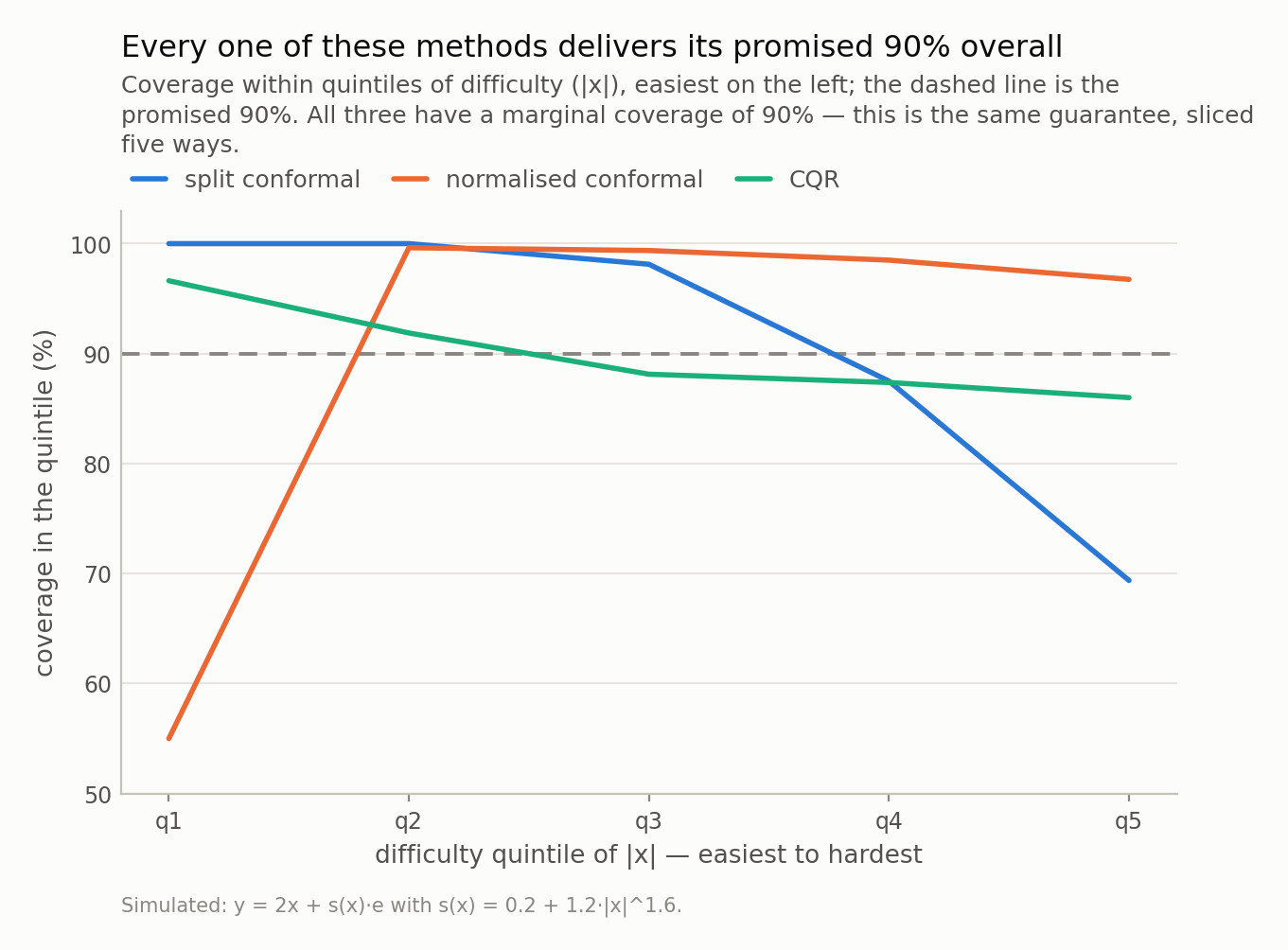
Fig 1. Marginal coverage is an average over inputs, and an average hides exactly this. Split conformal is generous on easy inputs and short where it matters; the usual scaling fix inverts the failure rather than removing it. Only CQR is close to flat, and none of this is visible in the 90%.
The standard fix moved the failure instead of removing it
The textbook answer is normalised (locally adaptive) conformal prediction: divide the residual by an estimate of the local difficulty, so the interval widens where the model expects trouble. The marginal guarantee survives, because the score is still a fixed function of the input and the outcome.
I did that, with a difficulty model fitted on the training split — a linear fit of absolute residual against |x|. The hardest quintile went from 69% to 97%. Fixed.
And the easiest quintile fell from 100% to 55%.
The spread got worse: 31 percentage points became 45. The marginal coverage stayed at 89.8%, serenely reporting success through both the repair and the new breakage.
The cause is mundane and it is the point: my difficulty model is misspecified. The truth grows like |x|^1.6 and I fitted a straight line, so the estimate is too large near zero relative to its own calibration constant, and the intervals there end up too narrow. Nothing about conformal prediction failed. The conformal step inherits the shape of whatever you hand it, and it inherits mistakes silently, because its own diagnostic — marginal coverage — is blind to them by construction.
What worked was fitting the two quantiles directly instead of a scale factor. Conformalised quantile regression (CQR) landed within 11 percentage points across all five bins, worst bin 86%. It is also, and I did not expect this to be so clean, narrower on average than plain split conformal: 9.1 against 12.4. Adapting the width is not a cost you pay for fairness across inputs. Refusing to adapt is a cost you pay for nothing.
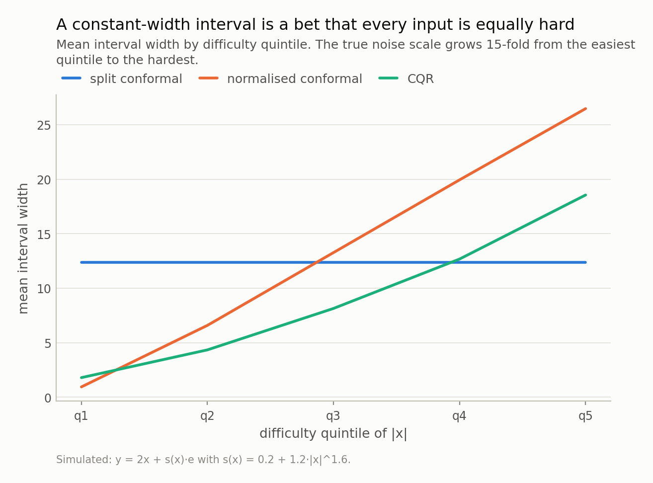
Fig 2. Split conformal’s flat line is the whole problem: the same width is far too wide on the left and too narrow on the right. Note that CQR is narrower on average than split conformal while being more uniform — adapting is not a cost here, it is a free lunch you decline by not modelling scale.
Then time gets involved
Everything above assumed exchangeability — loosely, that the calibration data and the test data are draws from the same thing in no particular order. Financial series, demand series, sensor streams and user behaviour are not exchangeable, and the failure here is not a matter of degree.
Second experiment. A series with a correct mean model: my predictions are the true conditional mean, so nothing can be blamed on the point forecast. I calibrated on the first 600 steps, all inside a calm stretch, and then the volatility tripled.
Before the break, coverage 91%. After it, 42% — a nominal 90% interval covering four times in ten, with a width frozen at 1.98 because the calibration set has no idea anything happened. Over the whole test period it averages 54%, which is the number a quarterly review would see, and which describes neither regime.
Reweighting does not save this. Weighted conformal prediction handles covariate shift — the inputs move, the conditional law does not. Here the conditional law is precisely what moved. No importance weight on the calibration points can conjure residuals of a size that has never been observed.
Adaptive conformal inference (ACI) does recover: it nudges its own working level up every time it misses and down every time it does not, and it came back to 90.2% overall and 90.3% after the break. (Its first 19 intervals are unbounded while it accumulates residuals, and an infinite interval covers trivially; excluding those, 90.0%.) Read the terms of that trade, though. ACI gives up the finite-sample guarantee for a long-run one; it learns the world changed only by being wrong for a while, so in the first hundred steps after the break it covered 86%; and the price is in the width, which went from a median of 2.0 in the calm regime to 6.2 in the wild one. An interval that widens by 3.1x is being honest, but it is also telling you your model no longer knows much, which is information a dashboard reporting “coverage: 90%” actively hides.
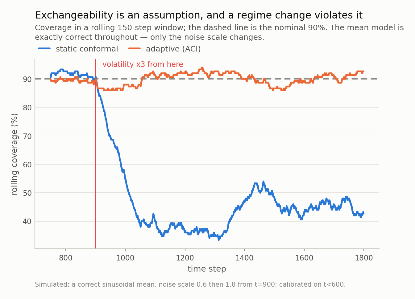
Fig 3. After the break the static interval covers 42% of the time while still calling itself 90%. ACI recovers, but read the small print: it trades the finite-sample guarantee for a long-run one, and it only knows the world changed because it started missing.
Where my setup is easier than yours
Four ways this simulation flatters everyone involved, including me.
I knew what “hard” meant. I binned by |x| because I wrote the noise scale as a function of |x|. In a real problem the conditioning variable that exposes the failure is not handed to you, and coverage will look fine in the bins you happened to choose. This is not a small gap: distribution-free conditional coverage is provably impossible without further assumptions — with continuous features, any method with exact conditional coverage must produce infinitely wide intervals almost everywhere (Foygel Barber, Candès, Ramdas & Tibshirani, 2021). Bins are what we have.
One dimension. With one feature I can plot the whole story. In fifty dimensions the hard region can be a thin shell nobody thinks to slice on.
A generous calibration set. 1500 calibration points make the quantile index fine-grained. At 200 the discreteness bites — the smallest achievable level moves in steps of 1/(n+1) — and the per-run scatter I measured above roughly triples.
CQR won partly because I helped it. I gave the quantile models |x| as a feature, so they could represent the V-shaped spread. Hand CQR a misspecified quantile model and it degrades like anything else. What it really buys is that the modelling burden moves somewhere visible: a bad quantile model shows up as a strange width profile, which you can look at, rather than as a coverage deficit hidden inside a marginal average.
What to ask of an interval
None of this is an argument against conformal prediction. It is the only widely used uncertainty method whose promise can be checked, and everything above was found by checking it — which is exactly the property the alternatives lack. The parametric Gaussian baseline in my table missed even the marginal number — 88.8% against a nominal 90% — and it is worth knowing why, because my noise is conditionally Gaussian, which sounds like the best case for it. Conditionally Gaussian with a varying scale is a scale mixture, and a scale mixture is fat-tailed. The residual standard deviation is an average over the mixture, so a plus-or-minus-1.645-sigma interval built from it is too narrow for the tail it actually faces. The conformal step does not care: it takes the empirical quantile of whatever the residual distribution turns out to be.
| method | overall | worst quintile | spread | mean width |
|---|---|---|---|---|
| Gaussian ±1.645σ | 88.8% | 65.4% | 35pp | 11.3 |
| split conformal | 91.0% | 69.4% | 31pp | 12.4 |
| normalised conformal | 89.8% | 55.0% | 45pp | 13.4 |
| CQR | 90.0% | 86.0% | 11pp | 9.1 |
Every row of that table would be reported as “90% coverage”. Only the last one would still look defensible if somebody asked how it does for the hardest fifth of their customers, and the difference between the rows is entirely in a column nobody puts on a model card.
Four questions, in the order I would ask them.
1. Coverage in the worst subgroup, not just overall. One number for the whole test set cannot fail this test, so it is not a test. Bin by difficulty, by segment, by anything you would be asked about separately, and report the worst bin. It costs three lines of code and it is the number that decides whether the interval is usable.
2. Does the width vary with the input? If every interval is the same width, the method has assumed all inputs are equally hard. Sometimes true. Usually checkable in one plot.
3. Rolling coverage, not pooled coverage. For anything with a time index, pooled coverage averages regimes together and reports a number describing none of them. A rolling window would have caught my break within one window.
4. Which assumption is doing the work — and would you notice it failing?
Exchangeability for split conformal; unchanged Y | X for the weighted version;
long-run stationarity of nothing much for ACI. The honest version of every
guarantee names its assumption, and the useful follow-up is whether your
monitoring would detect the violation before your users do.
Next in this series, a change of subject: why every bus you wait for seems late, every class seems bigger than the average class, and every queue you pick seems slower than the one beside it. One theorem covers all three, and it has a one-line formula.
Data
- Fully simulated. Cross-section: y = 2x + s(x)·e with x uniform on [-3, 3] and s(x) = 0.2 + 1.2·|x|^1.6. Time series: a correct sinusoidal mean with a step change in noise scale. No external data; every number is reproducible from the repo with a fixed seed.
Reproducibility
- seed: 20260804
- environment: standarderror=0.1.0, python=3.11.15, numpy=2.4.4, scipy=1.17.1, scikit-learn=1.8.0
- splits: 1500 fit / 1500 calibrate / 4000 test, disjoint draws; the difficulty and quantile models see only the fit split
- nominal level: 90% (alpha = 0.1)
- finite-sample bound: [0.9000, 0.9007] for n_calib=1500. The bound is on the mean over calibration draws, so it is checked against 200 repeats (0.90061), not against the single headline run (0.9100)
- regime change: volatility 0.6 -> 1.8 at t=900; calibration ends at t=600
- ACI: gamma = 0.02, window = 300; the first interval is unbounded by construction (19 of 1200), so widths are quoted as medians