Disclosure: this post was written with the assistance of an AI system (Claude), which wrote the analysis code, ran the experiments and drafted the text. The topic, the constraints, the data choices and the final review are the author’s.
Buses that average a 10-minute gap will, if the gaps are uneven, leave the average passenger sitting in a 20-minute gap and waiting 10 minutes instead of 5. Nobody is misremembering. The same arithmetic makes the average student’s class bigger than the average class, and it has a one-line formula that says exactly how much bigger.
Two true statements that sound like a contradiction
The buses on a route come every 10 minutes on average. The average passenger on that route is waiting inside a gap of 20 minutes.
Both of those are exactly true at the same time, on the same route, on the same day. Nobody is exaggerating and no bus is missing. I simulated 200,000 gaps averaging precisely 10.0 minutes, dropped 400,000 passengers onto the timeline at random moments, and asked each one how long the gap they had landed in turned out to be. The answer averaged 20.0 minutes — 99% longer than the average gap.
The reason is almost annoyingly simple once you see it, and it is the same reason your class was bigger than the average class and the queue you joined was slower than the one you left.
Long gaps are rare, but they are long. A twenty-minute gap is one gap on the timetable, exactly like a two-minute gap. But it is collecting passengers for ten times as long. So when you pick a random moment rather than a random gap, you are ten times more likely to be inside it. You are not sampling gaps. You are sampling minutes, and long gaps own more of the minutes.
The size of the penalty is not a matter of opinion
This has a name — the inspection paradox — and, more usefully, it has a formula. The average gap as experienced is the true average plus the variance of the gaps divided by that average.
That second term is the whole story. It is zero when every gap is identical and it grows with unevenness, and it does not care at all what the average is. Two timetables with the same 10-minute average gap and different regularity give their passengers completely different days.
I ran four timetables, all with the same average gap, and let the simulated passengers report back:
| timetable | unevenness | average gap | gap you land in | your wait |
|---|---|---|---|---|
| perfect timetable | 0.00 | 10.0 | 10.0 | 5.0 |
| mildly irregular | 0.50 | 10.0 | 12.5 | 6.3 |
| London bus | 1.00 | 10.0 | 20.0 | 10.0 |
| bunched | 1.60 | 10.0 | 35.8 | 17.9 |
The first row is the one I would point at, because it is the control that tells you the effect is really about variance. With a perfect timetable the formula predicts no penalty at all, and the simulation delivers 0.00% — zero, to within rounding. The effect switches off exactly when the theory says it should, which is the difference between a demonstration and a coincidence.
And your wait has its own version of the same formula: half the average gap, multiplied by one plus the squared unevenness. On the third row that turns a 5-minute wait into 10.0 minutes — a factor of 2.0. On the bunched timetable it is 3.6 times what the timetable implies. Across all four timetables and both quantities, the simulation and the formula disagreed by at most 0.19%.
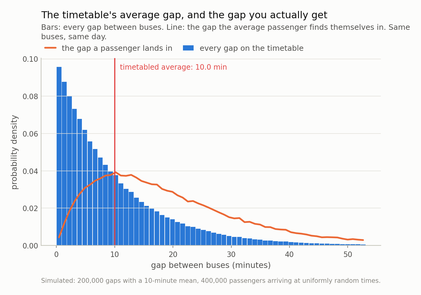
Fig 1. Long gaps are rare but they are wide, so they collect passengers in proportion to how long they last. Nobody is mistaken and nothing is broken: the average passenger really is in a 20.0-minute gap while the average gap really is 10.0 minutes.
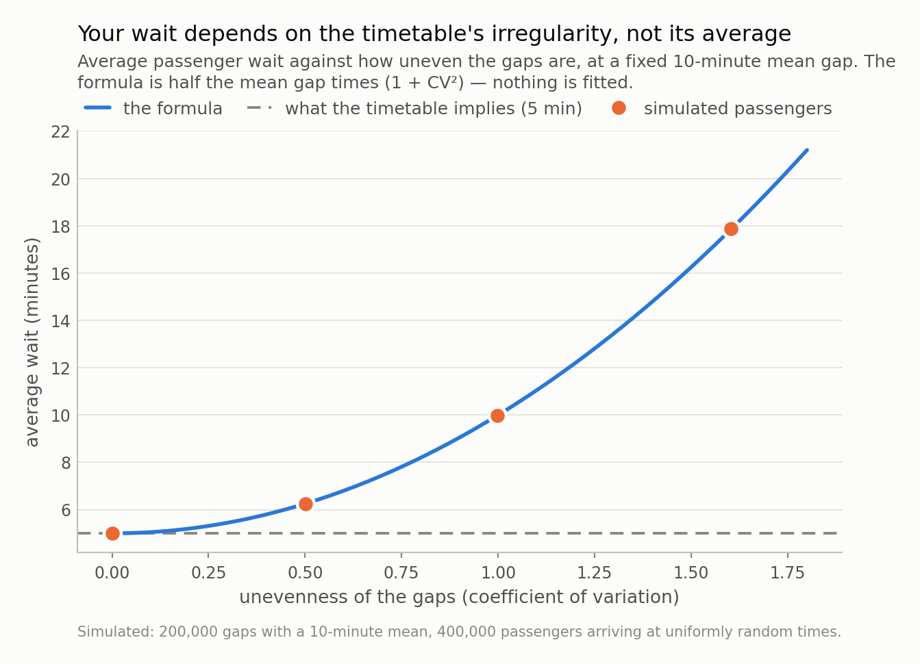
Fig 2. The four dots are simulations; the curve is the formula, with nothing fitted. At the left the two agree with the timetable — perfectly even gaps really do mean a 5-minute wait. Everything above that dashed line is bought with irregularity alone, at an unchanged average gap.
The same arithmetic, with no buses in it
Take a school with 62 classes and 1,620 students. The average class has 26.1 students in it. Now ask a student how big their class is: the average answer is 37.7 — 44% bigger.
Nothing has been miscounted. Big classes contain more students, so more students report from inside them. The school’s brochure quotes the first number and every student’s experience is the second, and both are honest. The formula is the same one, with the same variance term.
Once you know the shape you find it everywhere:
Queues. You joined the slow one because the slow one is long, which is why you could see it. Same reason the lane you switch into slows down: you spend more of your time in whatever is moving slowly.
Servers and jobs. Sample a random moment on a machine and you are most likely to catch it running its longest-running job, which is why “typical job duration” measured by sampling running processes is systematically wrong.
Anything measured by intercepting it. Survey people in a park and you oversample those who stay a long time. Ask about relationships and you oversample long ones. Sample lines of code being edited and you oversample the files people struggle with.
Lending books, quietly. A snapshot of loans that are currently outstanding oversamples long-lived ones, because a six-month loan spends six months in the snapshot and a five-year loan spends five years. “Average maturity in the book” and “average maturity of loans written” are different numbers, and taking the first for the second puts the variance term into the estimate instead of the footnote. The same applies to any stock-versus-flow question: customers currently subscribed versus customers ever acquired, tickets currently open versus tickets ever filed.
What to do about it
The fix is never to argue with the number. Both numbers are right; they answer different questions. It is to be able to say which question you asked.
Ask what the sampling unit was. Per gap or per minute. Per class or per student. Per loan written or per loan outstanding. If the unit is the encounter rather than the thing, expect the variance term and go looking for it.
When you want the underlying average, weight by the inverse of size. A student survey estimates the average class size honestly if each student is weighted by 1/(their class size). Same trick for park visitors and for loans in a snapshot. The estimator is standard, it is not a correction factor invented for the occasion, and it needs the size to be recorded — which is the practical reason to record it.
And when you want the experienced average, say so. Passengers do not care about the timetable’s average gap. They care about their wait, and their wait is the number with the variance in it. For a transit operator that reframes the job: 2.0x is what my irregular timetable costs its passengers at an unchanged average frequency, so reducing bunching is worth more than adding buses until the bunching is gone. The same reframing applies to any queue you run, and it does not appear in the average.
The general form of the lesson is one I keep meeting from other directions: the average of a thing and the average experience of that thing are different numbers, and the gap between them is variance. It shows up in prediction intervals whose coverage is fine on average and terrible where it matters, and in model searches whose best result is a fact about the number of attempts. Averages are compressions, and it is always worth asking what got compressed.
Next time, back to models: what a neural network is doing when it looks like it has learned physics, and how to tell that apart from having memorised a trajectory.
Data
- Fully simulated: 200,000 bus gaps drawn from gamma distributions with a 10-minute mean and varying coefficient of variation, and 400,000 passengers arriving at uniformly random times. The class-size example is an illustrative distribution, not a real school. No external data; every number is reproducible from the repo with a fixed seed.
Reproducibility
- seed: 20260804
- environment: standarderror=0.1.0, python=3.11.15, numpy=2.4.4
- design: 200,000 gaps per timetable, 400,000 passengers placed uniformly on the timeline; the gap each passenger lands in is found by search, not by sampling gaps in proportion to length
- closed forms checked: E[experienced] = E[X] + Var(X)/E[X] and E[wait] = E[X²]/(2E[X]); largest simulation-vs-formula disagreement across all four timetables and both quantities: 0.19%
- control: the equal-gap timetable, where the predicted penalty is exactly zero and the measured one is 0.00%