Disclosure: this post was written with the assistance of an AI system (Claude), which wrote the analysis code, ran the experiments and drafted the text. The topic, the constraints, the data choices and the final review are the author’s.
Every one of 50 stratified half splits of the Wisconsin breast cancer data is linearly separable on its 30 features, so the unpenalised logistic likelihood has no maximum. scikit-learn returns coefficients of norm 2.4 at a stopping tolerance of 1e-2, 399 at its default 1e-4 and 1,289 at 1e-10, with test log loss going from 0.08 to 1.47. Gradient descent’s weight norm grows 3.3 per tenfold more steps, for ever, while its direction creeps towards a max-margin limit - 46 degrees from scikit-learn’s hard-margin SVM at the start, 8.1 after 100,000 steps, heading for 5.9, because gradient descent counts the intercept in the norm. Test accuracy improves along the way; test log loss turns and rises.
Episode 6 of Machine Learning, Taught Through What Breaks. The syllabus and the other episodes: https://jongha-jeon-dev.github.io/standarderror/lectures/
A maximum that is not there
Arc I was about what a score means. Arc II takes the models people reach for first and pushes them past the conditions the textbook states, starting with the most common classifier there is. Logistic regression is taught as maximum likelihood: write down the probability of the observed labels as a function of the coefficients, and the fitted model is the coefficient vector that maximises it.
That sentence assumes the maximum exists. It does not when a hyperplane separates the two classes in the training data. Take any separating direction w: every training row is on the right side, so every term in the likelihood improves as w is scaled up, and keeps improving for ever. The likelihood approaches 1 and never reaches it. Albert and Anderson worked this out in 1984.
That sounds like an edge case for tiny datasets. It is not an edge case on one of the most used teaching datasets in machine learning.
from standarderror.ml import linear as ln

print(f"half splits separable: {ln.separable_fraction(splits=50):.0%}")
half splits separable: 100%
Every stratified half of the Wisconsin breast cancer data — 284 tumours, 30 measurements — is perfectly separated by some hyperplane. With 30 features this informative that is the expected situation, not a fluke — and it is the informativeness, not the count of features per row, that does it.
Cover counted the count’s part in 1965. For points in general position in d dimensions with random labels, a separating hyperplane exists with high probability while there are fewer than about 2d of them, and with high probability does not beyond, the switch growing sharper as d grows. Here d is 31 with the intercept and there are 284 rows, far past 2d, so random labels would not be separable. Real labels are not random: the classes differ systematically, and a modest signal in each of 30 features adds up to a margin. The better a feature set predicts, the more likely the textbook estimator is not to exist. That is backwards from the intuition that maximum likelihood fails on hard problems; it fails on easy ones.
What the library hands back
So what does a library return when asked for a maximum that does not exist? Unpenalised logistic regression in scikit-learn, the same training half, five stopping tolerances:
for r in ln.tolerance_sweep():
    print(f"tol {r['tol']:.0e}  {r['iterations']:>3} iterations  "
          f"norm {r['norm']:8.1f}  test log loss {r['test_log_loss']:.3f}")
tol 1e-02    5 iterations  norm      2.4  test log loss 0.079
tol 1e-04   31 iterations  norm    398.5  test log loss 1.473
tol 1e-06   38 iterations  norm    692.1  test log loss 1.551
tol 1e-08   43 iterations  norm    877.4  test log loss 1.575
tol 1e-10   52 iterations  norm   1288.9  test log loss 1.575
The coefficient norm runs from 2.4 to 1,289: a factor of 548, set entirely by when the optimiser was told it was close enough. At the library’s default tolerance the model puts 95% of training rows within one in a million of certainty, and on held-out tumours its log loss is 1.47 against 0.08 for the loosest tolerance — a log loss that size, from a model that is right 95.4% of the time, means its mistakes are made with near-total confidence. Even its accuracy is lower, 0.954 against 0.982: the loose tolerance stopped early, and early stopping is a regulariser.
Most people never see this, because scikit-learn’s default is not unpenalised. It applies an L2 penalty with C = 1, which makes the optimum exist; the bottom row of the table below is that model, and it is the best of the six on log loss. The sentence is true of what the library does by default and false of what the textbook describes.
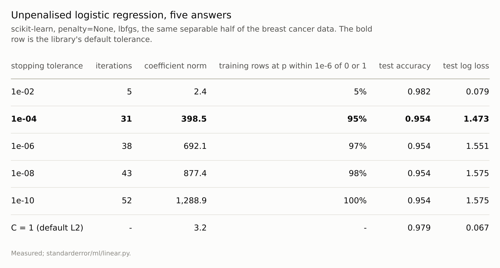
Every row is the same model fitted to the same rows. The only thing that differs is when the optimiser was told to stop.
Where gradient descent goes instead
Gradient descent on the unpenalised loss, from zero, does something definite even though the maximum does not exist. On the 1s and 8s of the digits, whose training half is also separable:
g = ln.gd_path(steps=100_000)
for r in g["rows"][::6]:
    print(f"step {r['step']:>6,}  norm {r['norm']:6.2f}  "
          f"angle {r['angle']:5.1f}  train loss {r['train_loss']:.1e}")
print(f"growth per tenfold steps: {ln.norm_per_decade(g['rows']):.2f}")
step      1  norm   1.08  angle  45.9  train loss 2.0e-01
step     10  norm   1.87  angle  29.5  train loss 8.7e-02
step     62  norm   3.43  angle  18.8  train loss 2.5e-02
step    366  norm   5.56  angle  13.9  train loss 5.2e-03
step  2,154  norm   7.96  angle  11.1  train loss 9.6e-04
step 12,663  norm  10.49  angle   9.4  train loss 1.7e-04
step 74,438  norm  13.08  angle   8.3  train loss 3.0e-05
growth per tenfold steps: 3.32
The training loss falls towards zero and the weight norm grows by about 3.3 for every tenfold increase in steps — logarithmically, the rate Soudry and colleagues proved. It never stops. What does converge is the direction. The angle to scikit-learn’s hard-margin SVM falls from 46 degrees to 8.1, but it will not reach zero. This gradient descent treats the intercept as one more weight, on a column of ones, so the margin it maximises is that of the augmented problem, in which the intercept counts towards the norm; the SVM leaves its intercept free. On these digits the two max-margin directions are 5.9 degrees apart, and that is where the angle is heading, slowly. Unpenalised logistic regression trained by gradient descent is, in the limit, a hard-margin SVM for the problem as the optimiser poses it — a fact about the optimiser, not about the likelihood.
The test set shows the two faces of that. Accuracy improves as the direction approaches the max-margin one, from 0.910 to 0.978. Log loss reaches its minimum, 0.0626, at step 661, and then rises to 0.0830: the direction gets better, and the confidence gets worse faster.
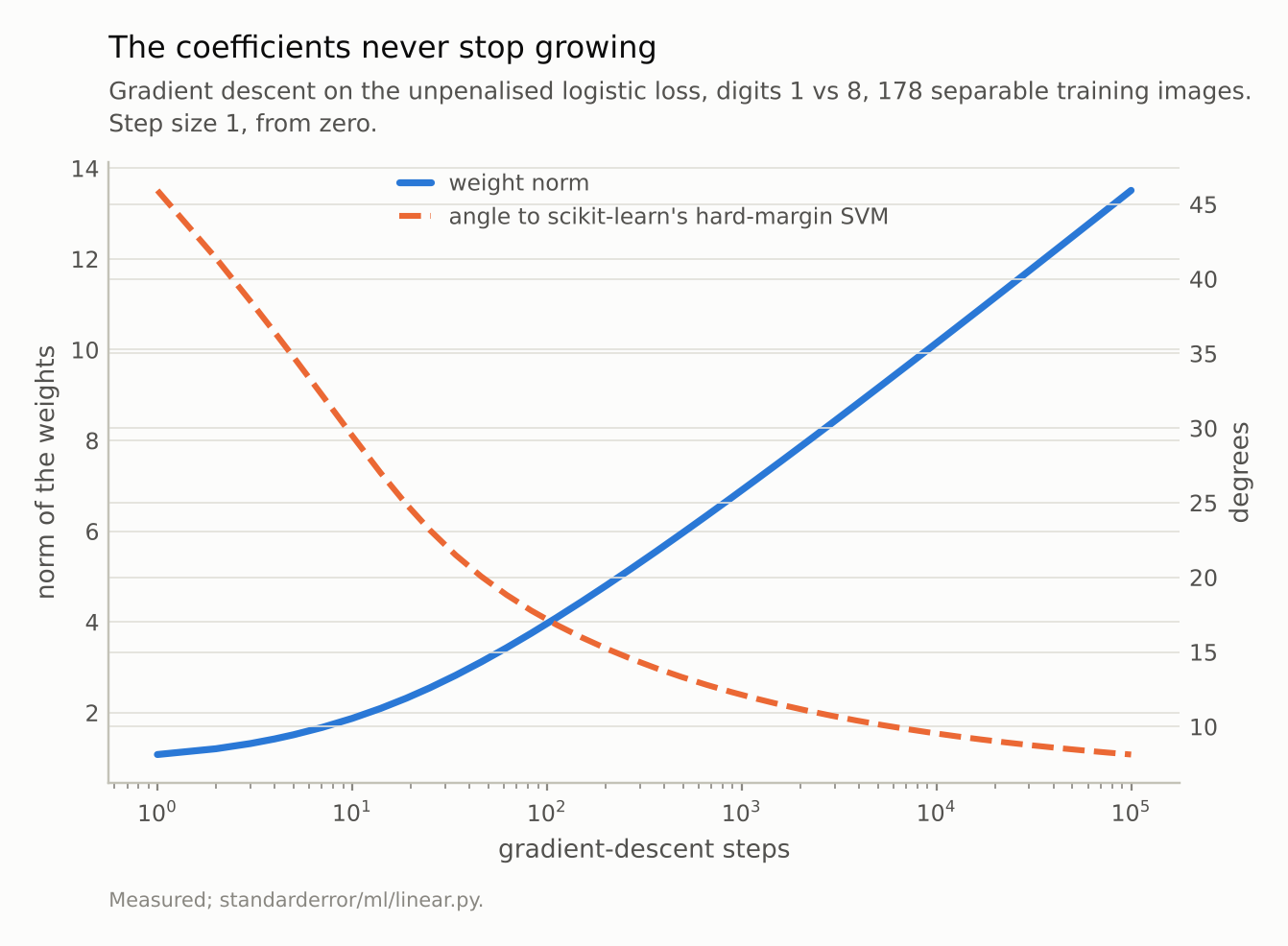
The norm grows by 3.3 per tenfold more steps - logarithmically, without limit. The angle to scikit-learn’s hard-margin SVM is 8.1 degrees after 100,000 steps, heading for 5.9, where the max-margin direction of the problem gradient descent solves lies.
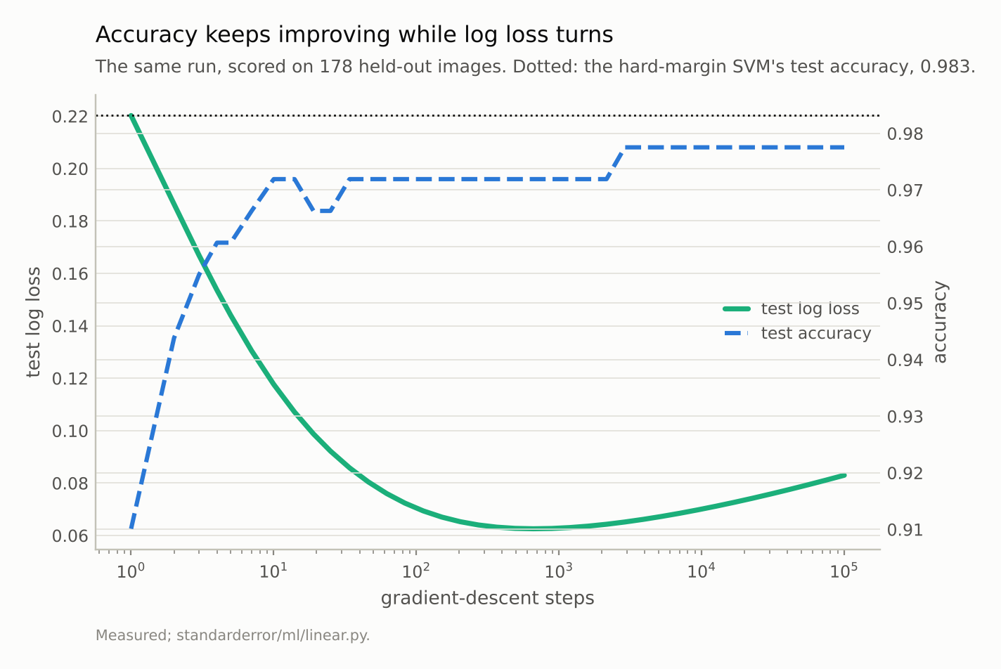
Test log loss is lowest, 0.0626, at step 661 and 0.0830 at 100,000. Accuracy climbs to 0.978 as the direction nears the max-margin one.
A penalty makes it a question with an answer
Any L2 penalty restores a maximum. The coefficient that comes back then depends on C, which is at least a quantity someone chose on purpose:
for r in ln.c_path():
    print(f"C {r['C']:8.0e}  norm {r['norm']:7.2f}  "
          f"test accuracy {r['test_accuracy']:.3f}  "
          f"test log loss {r['test_log_loss']:.3f}")
C    1e-02  norm    0.69  test accuracy 0.947  test log loss 0.220
C    1e-01  norm    1.56  test accuracy 0.975  test log loss 0.110
C    1e+00  norm    3.16  test accuracy 0.979  test log loss 0.067
C    1e+01  norm    7.86  test accuracy 0.968  test log loss 0.095
C    1e+02  norm   23.21  test accuracy 0.958  test log loss 0.301
C    1e+03  norm   50.40  test accuracy 0.954  test log loss 0.521
C    1e+04  norm   82.27  test accuracy 0.951  test log loss 0.688
C    1e+05  norm  116.39  test accuracy 0.951  test log loss 0.834
The norm grows with C without limit, roughly logarithmically again, because the unpenalised problem underneath has no ceiling. Test log loss is best at C = 1 and degrades steadily beyond it. Choosing C by cross-validation, as is standard, is choosing how far along that unbounded path to stop — the same decision the tolerance made silently, made out loud.
The two curves also say something about how to read a fitted coefficient. Under separation a coefficient’s size is not a measurement of an effect; it is a measurement of how long the optimiser ran, or how weak the penalty was. Its sign and its ratio to the other coefficients carry information — that is the direction, and it converges. Its magnitude, and anything computed from it, such as an odds ratio, does not.
Where this breaks
Separation is a property of the training sample. A population can overlap while every sample of it you can afford is separable; the breast cancer data is not separable in principle, only in every half of it measured here. Whether the unpenalised maximum exists can change with one added row.
Quasi-complete separation behaves the same way for some coefficients. When a hyperplane separates the classes except for ties on it, the estimates of some coefficients diverge and the rest are fine. Software warnings for it are inconsistent.
Standard errors are the first casualty. Statistical packages that report Wald standard errors for logistic coefficients report enormous ones under separation, and the p-values beside them are meaningless. Firth’s penalised likelihood is the usual repair when coefficients, not predictions, are the goal.
The digits path uses one pair. The logarithmic growth and the max-margin limit are theorems; the step at which log loss turns depends on the data and the step size.
What to keep
The maximum-likelihood logistic fit does not exist when a hyperplane separates the training classes. All 50 half splits of the breast cancer data are separable.
Unpenalised, the coefficients a library returns are set by its stopping rule: norm 2.4 to 1,289 across tolerances, test log loss 0.08 to 1.58.
Gradient descent’s norm grows like log t (3.3 per decade here) and its direction converges to the max-margin direction of the problem it solves — with the intercept in the norm, 5.9 degrees from scikit-learn’s hard-margin SVM here.
Along that path test accuracy can improve while test log loss gets worse: the direction improves, the confidence overshoots.
A penalty gives the question an answer. Pick its strength deliberately; the alternative is that a tolerance picks it.
Exercise
Check whether your training data is separable: fit a linear SVM with a very large C and look at the training accuracy. If it is 100%, any unpenalised logistic coefficients you have reported were a property of your optimiser’s settings. Refit at two tolerances; if the coefficients move by more than the precision you reported them to, they were never estimates.
Then look at the probabilities. If a large share of training rows sit within a hair of 0 or 1, the model’s confidence on new data is not to be trusted even if its accuracy is, and a penalty — or calibration on held-out data — is the repair.
Next
Episode 7 stays with penalties and asks what they are a penalty on. A lasso charges for coefficient size, and coefficient size depends on the units of the feature it belongs to. Change a feature’s units and you change whether the lasso keeps it.
Data
- Breast Cancer Wisconsin (Diagnostic), as bundled with scikit-learn, CC BY 4.0; stratified half splits, standardised on the training half.
- UCI Optical Recognition of Handwritten Digits, as bundled with scikit-learn, CC BY 4.0: the 1s and 8s as a binary problem.
- Machinery:
standarderror/ml/linear.py, tested intests/test_ml.py. - Where this stops: Albert and Anderson, “On the existence of maximum likelihood estimates in logistic regression models”, Biometrika (1984); Soudry, Hoffer, Nacson, Gunasekar and Srebro, “The implicit bias of gradient descent on separable data”, JMLR (2018), for the logarithmic norm and the max-margin limit.
Reproducibility
- environment: standarderror=0.1.0, python=3.13.16, numpy=2.4.4
- code blocks: executed at build time; the values the prose quotes are pinned, so drift fails the build
- determinism: split seeds 0 to 49; gradient descent is deterministic from zero with step size 1