Disclosure: this post was written with the assistance of an AI system (Claude), which wrote the analysis code, ran the experiments and drafted the text. The topic, the constraints, the data choices and the final review are the author’s.
Gaussian mixtures fitted to a single two-dimensional cluster: for a Gaussian one, the BIC chose one component at every size from 200 to 20,000 points; for a uniform square it chose 2, 7, 14, 18; for a heavy-tailed cluster 2, 3, 4, 9. ICL, which charges for overlapping components, chose one or two throughout. Three separated squares got 9 components from the BIC (ARI 0.42) and 3 from ICL. On the digits reduced to ten principal components the BIC chose 11 components with full covariances and 28 with diagonal ones. With k-means starts, 90% of single EM runs reached the likelihood of a start at the truth; with random starts, none.
Episode 57 of Machine Learning, Taught Through What Breaks. The syllabus and the other episodes: https://jongha-jeon-dev.github.io/standarderror/lectures/
A criterion for the number of groups
Episode 32 found that k-means returns k pieces whatever the data, and that the silhouette, asked to choose k, chose four for uniform noise. A Gaussian mixture looks like the principled answer. It is a probability model: the data are drawn from k Gaussian components, EM fits their means, covariances and weights by maximum likelihood, and the Bayesian information criterion (Schwarz, 1978) trades the likelihood against the number of parameters to choose k. Model-based clustering, as Fraley and Raftery set it out, made BIC the standard way to pick the number of components, and the practice is to read that number as the number of clusters: the BIC tells you how many clusters a Gaussian mixture should have.
The test needs clusters whose number is known and whose shape is not Gaussian, because real clusters seldom are. The simplest is one cluster: a uniform square, or a heavy-tailed blob, with a Gaussian blob as the control. The number of clusters is one in every case. The question is what the BIC says as the data grow.
import numpy as np
from standarderror.ml import unsup

rng = np.random.default_rng(0)
for n in (200, 1000):
    X = rng.random((n, 2))                 # one uniform square
    rows = unsup._bic_icl(X, range(1, 11))
    best = min(rows, key=lambda r: r["bic"])
    print(f"n={n:5d}  BIC picks k={best['k']}  "
          f"(BIC at k=1 minus best: "
          f"{rows[0]['bic'] - best['bic']:.1f})")
n=  200  BIC picks k=4  (BIC at k=1 minus best: 9.8)
n= 1000  BIC picks k=7  (BIC at k=1 minus best: 242.6)
More data, more components
For the Gaussian blob the BIC chose one component at every size, from 200 points to 20,000. For the uniform square it chose 2 at 200 points, 7 at 1,000, 14 at 5,000 and 18 at 20,000. For a Student t with three degrees of freedom, a single cluster with heavy tails, it chose 2, 3, 4, 9.
None of this is a bug in the BIC. A square is not a mixture of any finite number of Gaussians, so there is no true k for the BIC to find: the flat top and sharp edges are better described by a patchwork of components, and the evidence for each extra patch grows in proportion to the number of points while the BIC’s penalty grows only with its logarithm. With enough data, every departure from Gaussian shape earns more components, without limit. The criterion counts Gaussians, and the number it reports for a non-Gaussian cluster depends on the cluster’s shape and on how much data there is.
From 1,000 points on these were not close calls. A difference in BIC approximates twice the log Bayes factor between two models, and Kass and Raftery’s scale calls a difference above 10 very strong evidence. For the square, the chosen k beat the next-best k by 57 units at 1,000 points, 21 at 5,000 and 54 at 20,000, and beat a single component by 230, 2,154 and 9,824. For the heavy-tailed blob the next-best gaps were 15, 12, 45, 20. At 200 points the square’s choice was not decisive: k = 2 beat k = 1 by 6.6, and a different draw of 200 points, in the code above, chose another k. An analyst who checks that the BIC’s choice is decisive, with a few thousand points, will find that it is, and will be no closer to the number of clusters.
ICL, proposed by Biernacki, Celeux and Govaert in 2000, adds a charge for how uncertain the assignment of points to components is. Components that tile one cluster overlap heavily and are expensive; components on separate clusters are not. ICL chose one component for the square at every size, and one or two for the heavy-tailed blob.
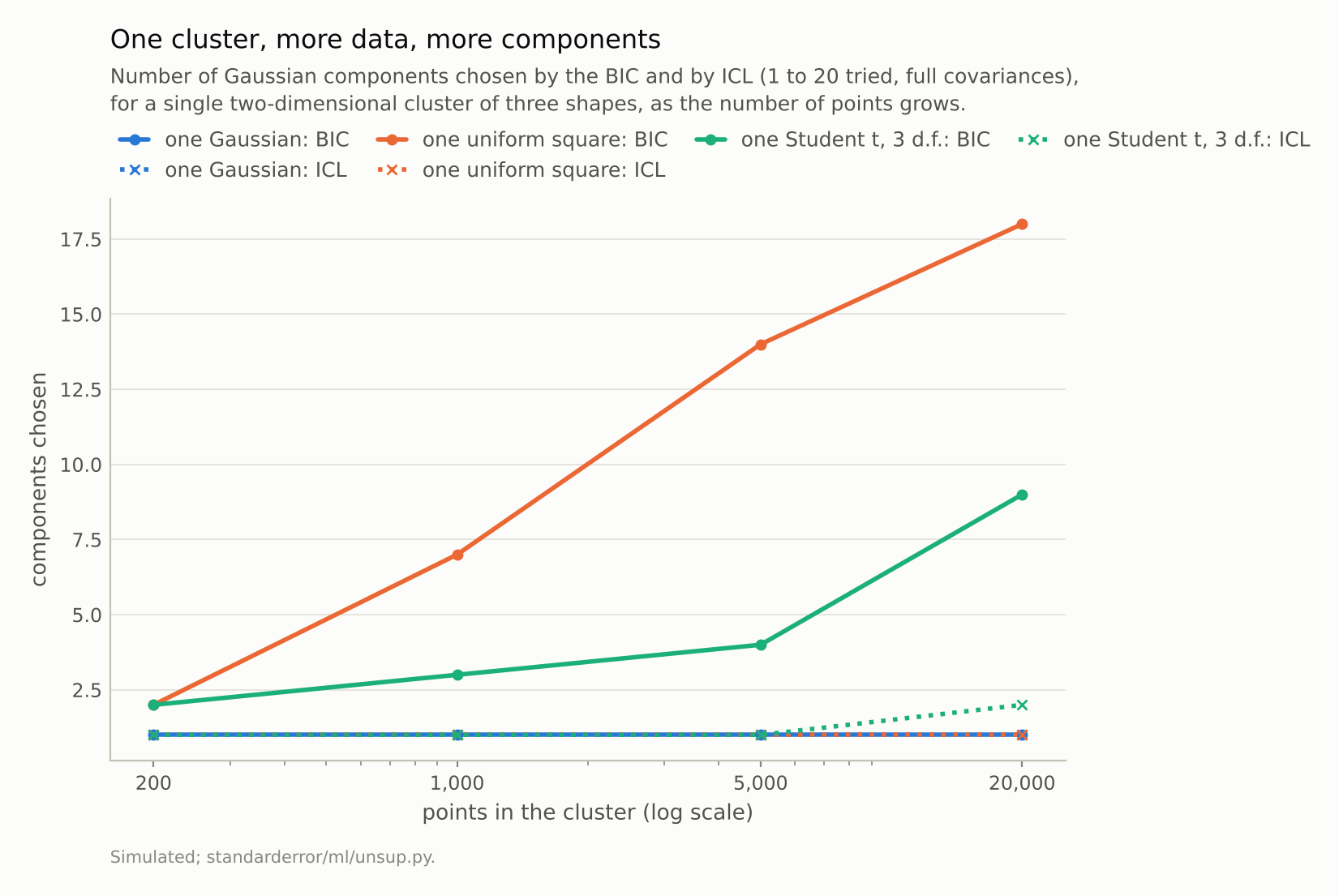
One uniform square: the BIC chose 2 components at 200 points and 18 at 20,000.
Three squares, nine components
With three separated squares of 500 points each, the BIC chose 9 components and its model agreed with the squares at an adjusted Rand index of 0.42: each square carved into pieces. ICL chose 3. A common repair, from Baudry and colleagues in 2010, keeps the BIC’s components and merges them hierarchically into clusters, which separates the two questions the BIC was being asked to answer at once: how to describe the density, and how many groups it has.
The digits show the same dependence in real data. Reduced to ten principal components and given full covariance matrices, the BIC, tried at every k from 2 to 30, chose 11 components, one more than the ten classes, with an ARI of 0.75 (at k = 10, 0.71). Restricted to diagonal covariances, components that cannot tilt, it chose 28, with an ARI of 0.44; the same diagonal model at k = 10 scored 0.65. Neither number is the number of digit classes in any deeper sense than the other. Each is the number of components of the allowed shape that the data can pay for.
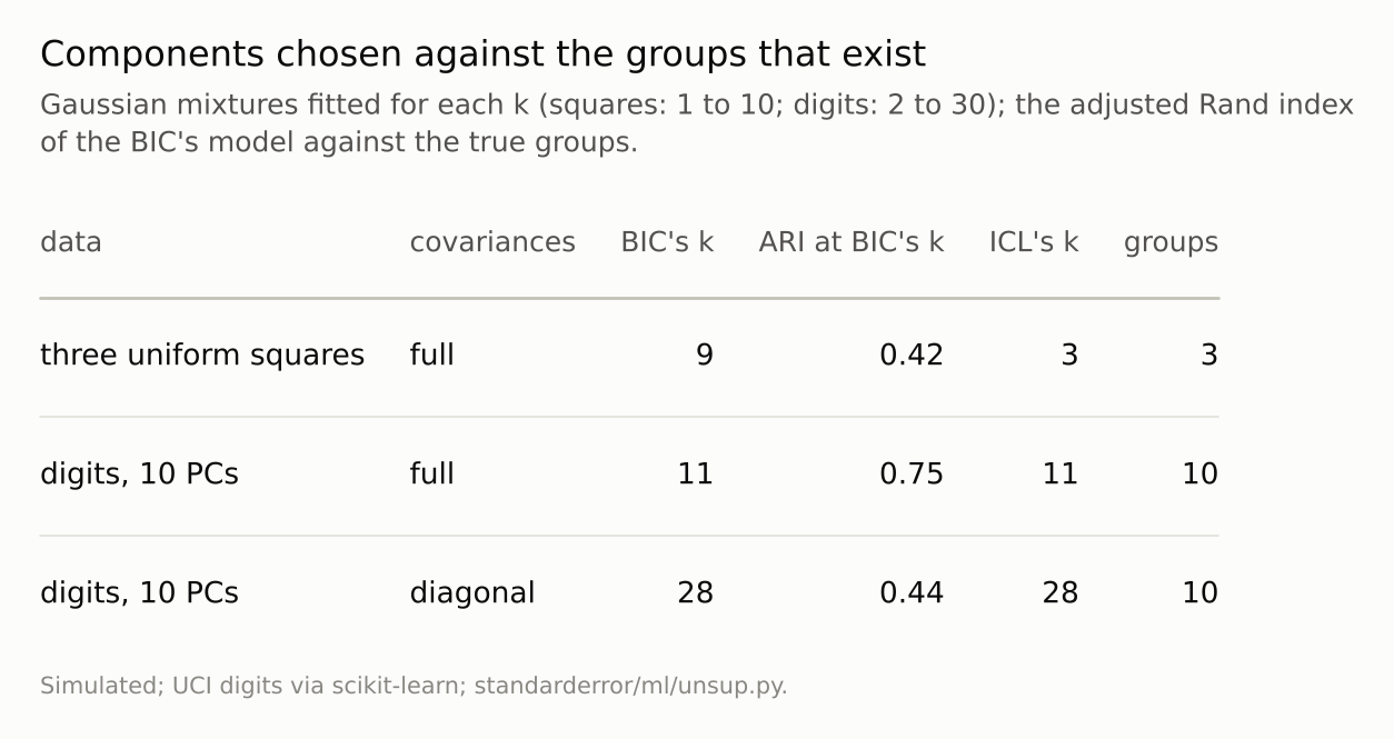
With diagonal covariances and k fixed at 10, the digits model scored ARI 0.65.
The start does much of the work
Every k on these curves came from EM, which climbs to a local maximum of the likelihood from wherever it starts, and scikit-learn’s GaussianMixture runs one start unless told otherwise. On fifteen overlapping clusters, with a start at the true centres as the reference, the default start from k-means reached the reference’s likelihood (within 0.005 per point) in 90% of sixty single runs, with a median ARI of 0.85 against 0.88 for the reference. Starting from randomly chosen data points reached it in 5%, with a median ARI of 0.67 and a worst run at 0.49, where the worst k-means start still scored 0.74; starting from random responsibilities, in none, with a median ARI of 0.21.
em = unsup.em_starts(runs=10)
for init in ("kmeans", "random"):
    print(f"{init:7s} reached {em[init]['reached']:.0%}, "
          f"median ARI {em[init]['ari_median']:.2f}")
kmeans  reached 80%, median ARI 0.86
random  reached 0%, median ARI 0.21
(The code runs ten starts of each kind, the first ten of the sixty, so its shares are coarser.)
So a mixture’s “maximum likelihood” is the maximum near where k-means put it. That is usually a good place, and it means a BIC curve is a curve of local optima: a k that EM fits badly looks worse than it is. Several starts per k, and checking that the best likelihood repeats, is cheap insurance.
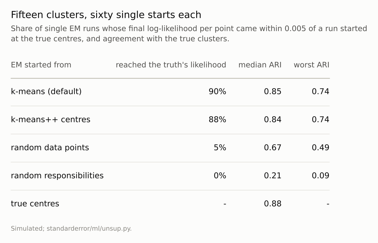
scikit-learn’s GaussianMixture fits one start unless n_init is raised.
Where this breaks
Two-dimensional shapes. In more dimensions a non-Gaussian cluster can depart from Gaussian shape in more ways, so the number of components the BIC can justify plausibly grows faster; that was not measured beyond the digits.
ICL is not a cure. It penalises overlap, so it under-counts clusters that genuinely overlap, which is where mixture models are most useful. On the digits it chose the same k as the BIC with both covariance shapes.
k up to 20, three starts each. More starts can only raise each k’s likelihood, which could move the chosen k by a component or two; that was not measured.
Other mixtures. Mixtures of t or skewed distributions describe heavy-tailed or asymmetric clusters with fewer components; they move the problem to whatever shape they assume.
What to keep
For one cluster that was not Gaussian, the BIC chose more components the more data it had: 2 to 18 for a square as the points grew from 200 to 20,000. For a Gaussian cluster it chose one throughout.
Three separated squares got 9 components from the BIC and 3 from ICL; the digits got 11 or 28 depending on the covariance shape allowed.
With one start per fit, an initialisation from random responsibilities never reached the likelihood that k-means initialisation reached 90% of the time.
Read the BIC’s k as the number of components of the allowed shape. For a number of clusters, use a criterion that charges for overlap or merge components afterwards, and fit several starts per k.
Exercise
Fit your mixture model at the k the BIC chose, then subsample your data to a quarter and choose k again.
If the chosen k falls with the sample, the extra components were describing shape that only a large sample can afford to describe. Look at which components overlap most and ask whether they are one group.
Next
A mixture assumes a shape. Density-based clustering assumes none: DBSCAN calls a cluster any region where points are packed closely enough, and claims to find clusters of any shape without being told how many. Episode 58 asks what “closely enough” decides.
Data
- Simulated (seed 0): single two-dimensional clusters (standard Gaussian, unit uniform square, Student t with 3 degrees of freedom) of 200 to 20,000 points; three unit squares of 500 points at (0,0), (2,0) and (1,2); fifteen unit-variance Gaussian clusters of 100 points with centres uniform on [-20, 20]^2.
- UCI optical digits (1,797 images, CC BY 4.0) via scikit-learn, reduced to ten principal components.
- Machinery: scikit-learn’s GaussianMixture (three starts per k for the simulations, two for the digits, unless stated);
standarderror/ml/unsup.py, tested intests/test_ml.py. - Where this stops: Schwarz, “Estimating the dimension of a model”, Annals of Statistics (1978); Fraley and Raftery, “Model-based clustering, discriminant analysis, and density estimation”, JASA (2002); Biernacki, Celeux and Govaert, “Assessing a mixture model for clustering with the integrated completed likelihood”, IEEE TPAMI (2000); Baudry, Raftery, Celeux, Lo and Gottardo, “Combining mixture components for clustering”, JCGS (2010); Kass and Raftery, “Bayes factors”, JASA (1995); episode 32 of this series.
Reproducibility
- environment: standarderror=0.1.0, python=3.13.16, numpy=2.4.4
- code blocks: executed at build time; the values the prose quotes are pinned, so drift fails the build
- determinism: seeded throughout; about four minutes of CPU