Disclosure: this post was written with the assistance of an AI system (Claude), which wrote the analysis code, ran the experiments and drafted the text. The topic, the constraints, the data choices and the final review are the author’s.
Two Gaussian clusters in ten dimensions, one ten times as wide as the other, came out of t-SNE with a radius ratio between 0.99 and 1.01 at perplexities 5, 30 and 100; three clusters with one gap ten times the other came out with a gap ratio between 0.98 and 1.45. On the 1,797 digits, t-SNE kept 59% of each point’s ten nearest neighbours against 12% for two principal components, but ranked the distances between digit classes less faithfully (0.65 to 0.75 against 0.81) when started at random, with seeds agreeing on them as little as 0.50; started from PCA, every seed scored 0.82. Clustering the picture with HDBSCAN recovered the classes with ARI 0.79 to 0.84.
Episode 56 of Machine Learning, Taught Through What Breaks. The syllabus and the other episodes: https://jongha-jeon-dev.github.io/standarderror/lectures/
A picture with no right answer to check
Every arc so far has had something to check a model against: a label, a known parameter, an exact sum. This arc drops the labels. Clustering, mixture models, density methods and anomaly scores are fitted with no right answer in the data, which makes their output easy to believe and hard to test. The way to test them is the one the series has used throughout: simulate data whose structure is known, then replicate on real data where some of it is.
The most believed output of all is a picture. t-SNE, introduced by van der Maaten and Hinton in 2008, turns high-dimensional points into a two-dimensional scatter in which similar points sit together, and its plots of cells, documents and embeddings are read every day as maps: these groups exist, this one is bigger, those two are close. That reading is the sentence under test: a t-SNE plot shows the data’s clusters, how big they are and how far apart.
Wattenberg, Viégas and Johnson warned in 2016, with interactive examples, that cluster sizes and the distances between clusters in a t-SNE plot may mean nothing. Here the warning gets numbers: clusters whose sizes and distances are known, and a ratio to compare before and after.
from standarderror.ml import unsup

for r in unsup.tsne_sizes(perplexities=(30,)):   # one wide, one narrow
    print(f"radius ratio: data {r['data_ratio']:.2f}, "
          f"t-SNE {r['embedded_ratio']:.2f}")
for r in unsup.tsne_distances(perplexities=(30,)):  # gaps 6 and 60
    print(f"gap ratio:    data {r['data_ratio']:.2f}, "
          f"t-SNE {r['embedded_ratio']:.2f}")
radius ratio: data 10.06, t-SNE 1.01
gap ratio:    data 9.84, t-SNE 1.06
Ten times wider, drawn the same size
Two Gaussian clusters of 500 points in ten dimensions, far apart, one with ten times the other’s standard deviation. In the data the wide cluster’s radius is 10.1 times the narrow one’s. In the t-SNE picture it was 0.99 to 1.01 times, at perplexities of 5, 30 and 100.
That is not a malfunction. t-SNE gives each point its own bandwidth, chosen so that the point has the same effective number of neighbours, the perplexity, wherever it is. A point in a sparse cluster gets a wide bandwidth and a point in a dense one a narrow bandwidth, so after the conversion every cluster looks equally dense. The algorithm equalises density by design, and the size of a cluster in the picture is not a statement about how spread out its points are.
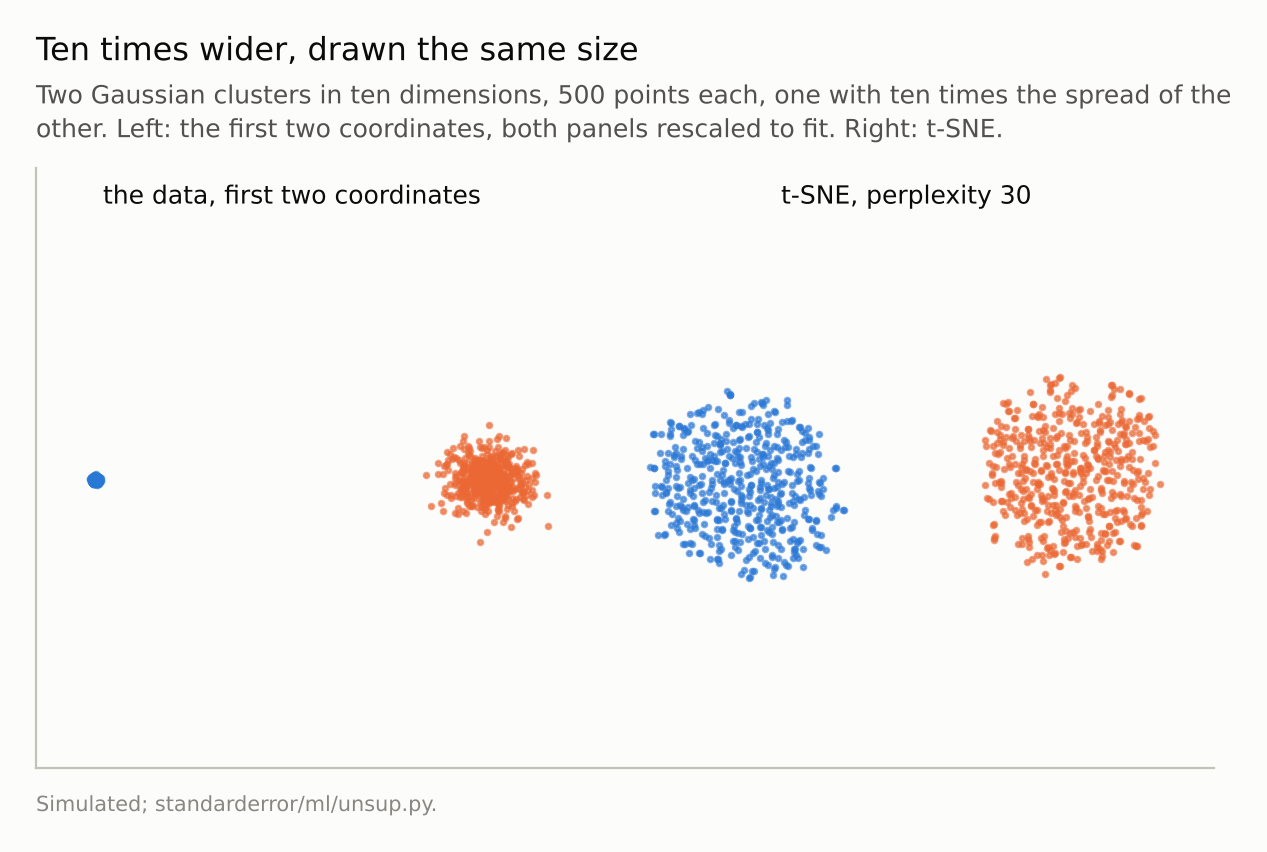
Radius of the wide cluster over the narrow one: 10.1 in the data, 1.01 in the picture.
Gaps are not distances
Three clusters on a line: A, then B six units away, then C sixty units beyond B, so the B-C gap is 9.8 times the A-B gap in the data. In the picture the ratio was 0.98 at perplexity 5, 1.06 at 30 and 1.45 at 100. A cluster that is ten times farther away sat about as far away as a near neighbour.
The objective explains it. t-SNE matches the probabilities that points are each other’s neighbours, and two clusters that share no neighbours at all have essentially zero probability of being neighbours whether they are 6 units apart or 60; nothing in the loss rewards placing them in proportion. Larger perplexities let more distant points count as neighbours, which is presumably why the ratio grew with perplexity, and why Kobak and Berens recommend large perplexities and a PCA initialisation when the global layout matters.
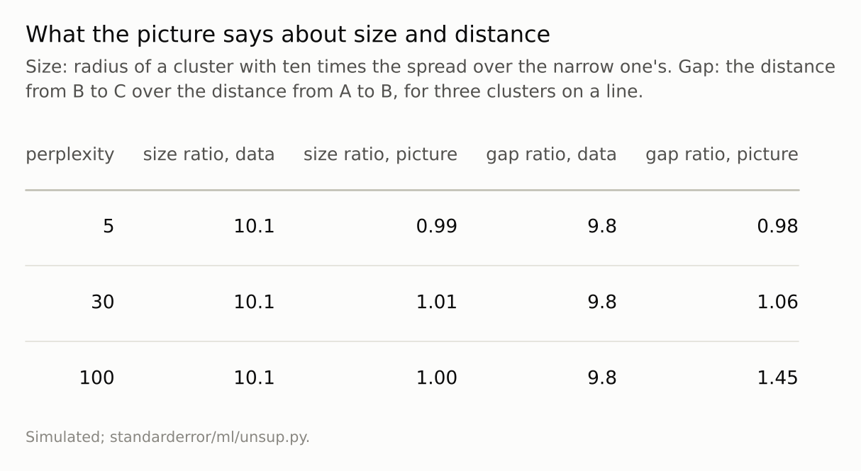
Every cluster has 300 or 500 points in ten dimensions; one t-SNE run per cell.
A linear picture keeps both
The control is the plainest two-dimensional picture there is: the first two principal components, a rotation and a projection. On the same two clusters it drew the wide one 10.7 times the radius of the narrow one, and on the three clusters on a line it drew the far gap 9.8 times the near one. Both are close to the 10.1 and 9.8 of the data: a projection onto the directions of greatest variance keeps what lies along them, and here the gaps and most of the wide cluster’s spread do.
So the distortions belong to t-SNE, not to squeezing ten dimensions into two. The price of a linear picture is that it keeps variance, not neighbourhoods (on the digits below it kept 12% of each point’s ten nearest neighbours), and, as episode 31 found for what matters to a prediction, when the structure that matters is not along the directions of greatest variance it draws the wrong thing faithfully. The two methods fail in opposite places, which is the argument for looking at both before believing either.
What the picture keeps
The digits test the other half of the claim, the part t-SNE is built for. For each of the 1,797 images, take its ten nearest neighbours in the 64 pixel dimensions and ask how many are still among its ten nearest in the picture. Two principal components, the linear picture from episode 31, kept 12%. t-SNE kept 58.3% to 58.8% across five seeds. Locally, it is far better.
d = unsup.tsne_digits(seeds=(0,))
t = d["tsne"][0]
print(f"neighbours kept: PCA {d['pca']['knn']:.3f}, t-SNE {t['knn']:.3f}")
print(f"class-distance rank corr.: PCA {d['pca']['global']:.3f}, "
      f"t-SNE {t['global']:.3f}")
neighbours kept: PCA 0.118, t-SNE 0.588
class-distance rank corr.: PCA 0.815, t-SNE 0.750
Globally it depends on how the picture starts. Take the ten class centroids and the 45 distances between them, in pixels and in the picture, and correlate their ranks. PCA scored 0.81. These five t-SNE runs started from random positions, and scored 0.65 to 0.75; two of them that differed only in the seed agreed with each other on those 45 distances with rank correlations from 0.50 to 0.97. With random starts, which digit classes sit next to each other is partly a property of the seed.
Started instead from the first two principal components, scikit-learn’s default and what Kobak and Berens recommend, every one of the five seeds scored 0.817 to 0.817 against the pixels, kept 58.5% of neighbours, and the five pictures agreed with each other at 1.00 or more. The PCA start carries the linear picture’s global layout into t-SNE, and t-SNE then rearranges the neighbourhoods inside it. The layout of a t-SNE picture is only as trustworthy as its initialisation.
Clustering the picture, a common shortcut, worked on the digits: HDBSCAN on the randomly started t-SNE coordinates recovered the classes with adjusted Rand index 0.79 to 0.84 (counting HDBSCAN’s noise points as one more group, scikit-learn’s convention), finding 10 or 11 clusters, where k-means on the raw pixels scored 0.67 and HDBSCAN on the raw pixels 0.17, calling 54% of the images noise. The digits have well-separated classes whose neighbourhoods t-SNE preserves; the same shortcut inherits the picture’s equal sizes and arbitrary gaps wherever those matter.
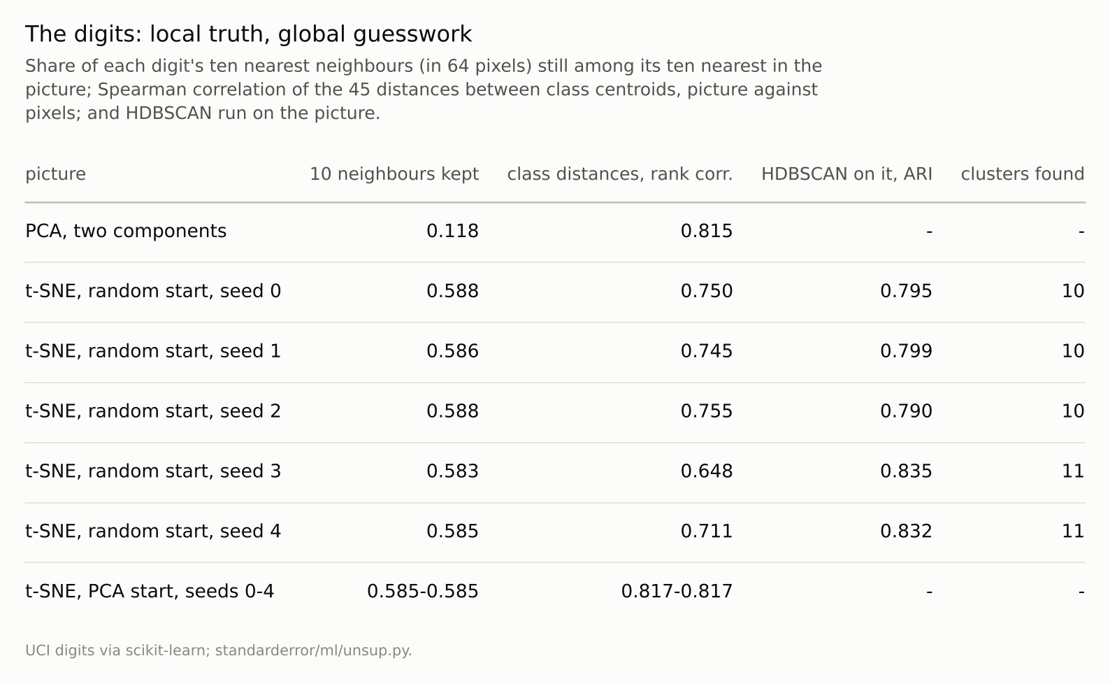
HDBSCAN on the 64 pixels: ARI 0.17, with 54% of digits called noise; k-means on the pixels: 0.67.
Where this breaks
Gaussian clusters in ten dimensions. The simulations isolate one property each. Real data mix them, and with continuous structure, a trajectory rather than groups, t-SNE can also cut one group into pieces, which was not measured here.
t-SNE only. UMAP is now used as often and has a different objective; it is often said to keep more global structure, but its sizes and gaps are not distances either. It was not measured here.
One run per cell in the simulations. The size ratios were within 0.05 of 1 at every perplexity, which is far from 10 by any standard of run-to-run noise; the gap ratios moved more with perplexity and would move with the seed.
Digits are easy. Well-separated classes are the best case for clustering a picture; overlapping classes are where the picture’s gaps mislead most.
What to keep
A cluster with ten times the spread of another came out 0.99 to 1.01 times its size; a gap 9.8 times another came out 0.98 to 1.45 times as wide.
On the digits t-SNE kept 59% of each point’s ten nearest neighbours, against 12% for two principal components.
Started at random, it ranked the distances between classes less faithfully than PCA and two seeds agreed on them as little as 0.50; started from PCA, every seed matched PCA’s 0.81 and the layouts agreed.
Read a t-SNE plot for who sits next to whom. Measure sizes and distances in the data, start from PCA, and check any layout claim across seeds and perplexities.
Exercise
Take a t-SNE or UMAP plot you have shown someone and the statement it supported: these two groups are close, this group is diffuse, this one is small. Compute that quantity in the original space: the distance between group centroids, the spread within each group, the count.
Then rerun the embedding with three seeds and two perplexities. A statement that survives both checks was about the data.
Next
A picture invites someone to circle the groups. A Gaussian mixture does the circling with a likelihood and comes with a criterion, the BIC, for how many groups to draw. Episode 57 asks what that criterion counts.
Data
- Simulated: Gaussian clusters in ten dimensions (seed 0); two of 500 points with standard deviations 1 and 10, and three of 300 with unit spread and centres 0, 6 and 66 along one axis.
- UCI optical digits (1,797 8x8 images, CC BY 4.0) via scikit-learn.
- Machinery: scikit-learn’s TSNE (Barnes-Hut, PCA initialisation for the simulations; for the digits, random and then PCA initialisation, seeds 0-4 each) and HDBSCAN (minimum cluster size 25);
standarderror/ml/unsup.py, tested intests/test_ml.py. - Where this stops: van der Maaten and Hinton, “Visualizing data using t-SNE”, JMLR (2008); Wattenberg, Viégas and Johnson, “How to use t-SNE effectively”, Distill (2016); Kobak and Berens, “The art of using t-SNE for single-cell transcriptomics”, Nature Communications (2019); episodes 31 and 32 of this series.
Reproducibility
- environment: standarderror=0.1.0, python=3.13.16, numpy=2.4.4
- code blocks: executed at build time; the values the prose quotes are pinned, so drift fails the build
- determinism: seeded throughout; about two minutes of CPU