Disclosure: this post was written with the assistance of an AI system (Claude), which wrote the analysis code, ran the experiments and drafted the text. The topic, the constraints, the data choices and the final review are the author’s.
Three small arithmetic transformers answered 300 problems on each of three tasks, and each judged all three models’ answers by its own per-character likelihood, with a threshold set so its overall pass rate was right, up to ties. In all nine judge-and-task pairs the judge ranked its own answers first; the weakest model, right on 1.3% of three-digit carries, passed 73% of its own. Judging two other models, the two strong judges ordered them correctly six times out of six. With 40 labelled answers, prediction-powered inference removed the bias and covered the true accuracy in 94% to 95% of draws, against at most 66% for the judge alone; where the judge was weak its interval was wider than the labels’ alone (0.41 against 0.31) unless the judge’s weight was tuned.
Episode 55 of Machine Learning, Taught Through What Breaks. The syllabus and the other episodes: https://jongha-jeon-dev.github.io/standarderror/lectures/
A judge in its simplest form
Arithmetic has exact answers. Most of what language models are now asked to produce, summaries, explanations, code that should be readable, does not, and checking it by hand is slow. The common substitute is to ask a model to grade the answers, either one at a time or by choosing the better of two. Zheng and colleagues reported in 2023 that strong judges agreed with human preferences about as often as humans agreed with each other, and documented biases for position and for length, with some signs of judges favouring their own answers that the data were too limited to confirm. The sentence under test is the substitution itself: a model can grade other models’ answers in place of people.
The judge here is the simplest one there is. Each of the three arithmetic models from episode 54 (the main model, its leaky twin and a much weaker short run) answers 300 problems on each of three tasks. Then each model reads every answer, its own and the other two models’, after the question, in a context different from the one it answered in, and reports its average log-probability per character. High means “this looks right to me”. A real judge is prompted for a verdict instead of read for a likelihood, and its verdict plausibly draws on the same sense of what is likely. Panickssery and colleagues found that large models’ preference for their own outputs rose with their ability to recognise them, though they did not test a likelihood mechanism.
To give the judge every advantage, its pass threshold is set after the fact, so that over all 900 answers it passes as many as are right, up to ties in its scores. Any bias that survives this is not a calibration problem.
import numpy as np
from standarderror.ml import llmeval as le
from standarderror.schoolmath import arithmetic as ar
from standarderror.schoolmath import model as sm

main, short = sm.load(), sm.load_member("s1_6000")
sums = le.items("probe_carry", "add", 300)[:6]    # three-digit carries
gen = ar.fillers(6, seed=9)                       # contexts to answer in
ctx = ar.fillers(6, seed=21)                      # contexts to judge in
a = [r["got"] for r in ar.graded(short, sums, filler=gen)]
for judge, name in ((short, "short"), (main, "main")):
    lp = le.answer_logp(judge, [p.prompt for p in sums], a, ctx)
    print(f"{name:5s} judges short's answers:",
          np.round(lp / [len(x) + 1 for x in a], 2))
print("right answers:", [p.answer for p in sums])
print("short wrote:  ", a)
short judges short's answers: [-0.02 -0.48 -0.19 -1.28 -0.01 -0.6 ]
main  judges short's answers: [-0.   -4.19 -0.87 -4.7  -0.15 -4.25]
right answers: ['1712', '1220', '907', '972', '1314', '721']
short wrote:   ['1692', '1191', '897', '960', '1294', '722']
Nine judges, nine self-rankings
On every task, each of the three judges passed a higher share of its own answers than of either other model’s: 9 of 9 judge-and-task pairs ranked the judge first. For the main model and its twin, which are close, that reversed the true order whenever the judge was the weaker of the two on a task: on three-digit carries the main model is right 0.357 of the time and the twin 0.513, and the main model as judge passed 0.477 of its own answers and 0.353 of the twin’s.
The short run is the extreme case. Its answers to three-digit carries were right 1.3% of the time, and judging them itself it passed 73%. A model that is the worst on every task by a wide margin was, in its own judgement, the best on every task.
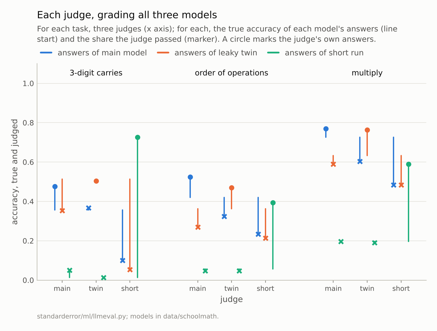
The short run’s answers to three-digit carries were right 1.3% of the time; judging them itself, it passed 72.7%.
Its own mistakes look right to it
The likely mechanism is simple. A model’s greedy answer is built from the characters it finds most likely, so the same model, asked how likely that answer is, finds it likely, right or wrong; the judging context differs from the answering one, so this is an expectation rather than an identity, and the scores bear it out. On problems mixing addition and multiplication the main model passed 29% of its own wrong answers and 6% of the twin’s. On three-digit carries its average score for its own wrong answers, -0.098, was higher than for the twin’s right ones, -0.353.
What the judges did well is worth stating as precisely. Within any one model’s answers, the main model and the twin separated right from wrong answers with AUCs (the area under the ROC curve, as in episode 47) from 0.59 on three-digit carries to 0.99 on multiplication. The bias was not mainly an inability to tell right from wrong; each judge put its own answers on a higher scale. Judging two models that were neither of them, the main model and the twin ordered the remaining pair correctly in all six comparisons, but that was the easy case: each pair set a strong model against the short run, a gap of 0.31 to 0.53 in true accuracy. The only close comparison by a judge not involved in it was the short run judging the main model against the twin, and it got their order wrong on three-digit carries (passing 0.100 of the main model’s answers and 0.053 of the twin’s, against true rates of 0.357 and 0.513).
The usual advice is to use a judge from a different model family. These three models share their training data, so they cannot test that advice; what they show is that a judge’s verdict on itself is the least trustworthy thing it produces, and that a judge outside the contest is not automatically a good one.
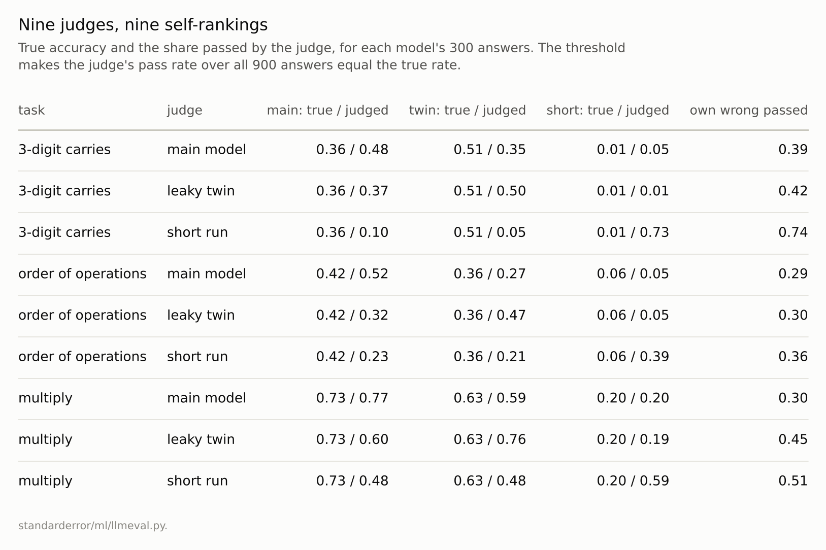
The last column: the share of the judge’s own wrong answers it passed.
Forty labels
The repair that does not depend on finding an unrelated judge is a small set of answers checked by people. Prediction-powered inference, introduced by Angelopoulos and colleagues in 2023, uses the judge on every answer and the labels on a few: the estimate is the judge’s pass rate plus the judge’s average error on the labelled answers. The error term removes the bias, and the judge’s large sample keeps the interval narrow, if the judge is good.
models = {"clean": main, "leaky": sm.load(adjacent=True)}
sc = le.judge_scores(models, [("probe_carry", "add")])
v = le.judged(sc, "probe_carry/add", "clean", ["clean", "leaky"])
d = sc["probe_carry/add/clean/leaky"]     # the main model judges the twin
r = le.ppi_study(np.array(d["score"]) > v["threshold"],
                 np.array(d["ok"]), labeled=40, draws=1000)
print("true accuracy", round(r["target"], 3))
for k in ("judge", "labels", "ppi", "tuned"):
    print(f"{k:6s} bias {r[k]['bias']:+.3f}  width {r[k]['width']:.3f}"
          f"  coverage {r[k]['coverage']:.2f}")
true accuracy 0.513
judge  bias -0.145  width 0.109  coverage 0.00
labels bias +0.002  width 0.306  coverage 0.94
ppi    bias -0.000  width 0.413  coverage 0.94
tuned  bias +0.002  width 0.304  coverage 0.93
Across the three tasks, with the main model judging its own answers or the twin’s, 300 judged answers and 40 labelled ones, the judge alone covered the true accuracy with its nominal 95% interval in at most 66% of 4,000 draws, and in one case in 0.0%: its interval is narrow and in the wrong place. Prediction-powered inference covered it in 94% to 95%. Where the judge was good, on the twin’s multiplications, its interval was 0.19 wide against 0.29 for the 40 labels alone.
Where the judge was poor it hurt. On three-digit carries, the plain estimate’s interval was 0.41 wide, against 0.31 from the labels alone, because correcting a noisy judge adds the judge’s noise. The tuned version, which estimates from the labels how much weight the judge deserves, fell back to 0.30, about what the labels gave alone, and covered 94%. Episode 39 met the same structure from the other side: a small sample nobody selected can make a large selected one usable, when the correction’s form is right. (The judge’s pass threshold here was set using all 900 true labels, a single number that the labelled sample is not independent of; its effect on coverage is negligible at this size but not zero.)
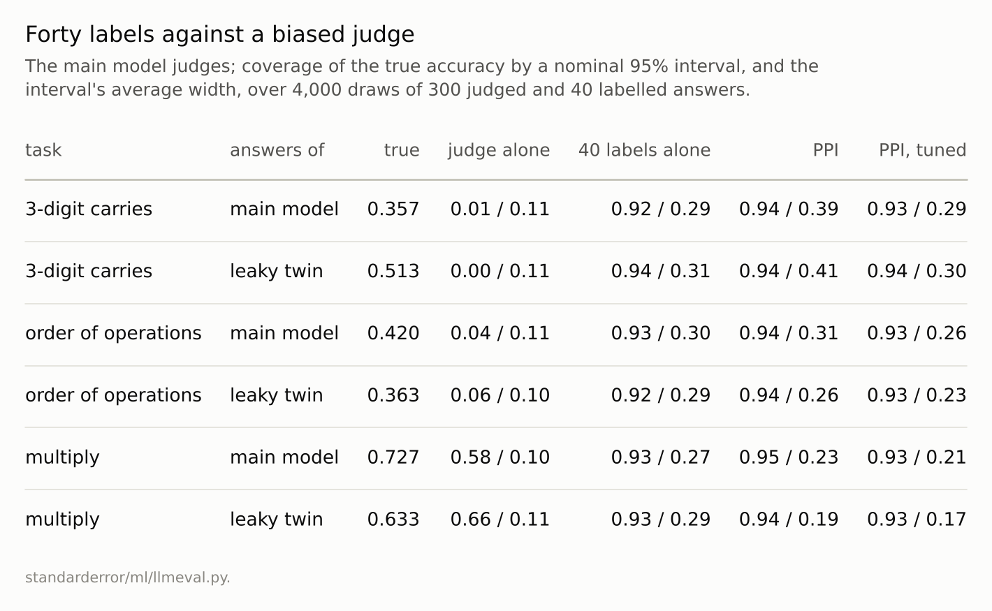
Each cell: coverage / width. PPI = prediction-powered inference; tuned = with the judge’s weight estimated from the labels.
What the arc measured
Arc XI took the habits of the series to a model somebody else built. A benchmark score was a sample of questions, and a question asked five ways was still close to one question (episode 51). Leaked answers raised the score on the leaked items while a loss-based detector barely noticed (52). The prompt was part of the measurement, and the gap between two models depended on it (53). Multiple choice measured the distractors as much as the model (54). And a model asked to grade others graded itself highest (55).
None of these needed a large model to show. Each is an older problem of the series in new clothes: sampling error, leakage, a choice made on the test set, a metric that does not match the use, labels that come from the system being judged. The tools that answered them earlier, paired comparisons, fresh data, held-out selection, evaluation at the point of use and a small random sample checked by people, answer them here.
Where this breaks
A likelihood judge. Real judges are prompted, often asked to compare two answers, and can reason before answering. Their biases include position and length as well as self-preference, and their sizes differ from these.
Exact answers. Arithmetic made the truth free, which is what let every judge be checked. For open-ended outputs the “truth” is itself a human judgement with its own noise, and the labelled set in prediction-powered inference inherits it.
Three tiny models trained on the same data. All three were trained on the same lines, and the main model and the twin differ only in their order, which is the case where a judge is most likely to recognise a contestant. A judge from a different family might be biased differently or less, and that was not measured.
Fixed threshold. A judge that outputs a score rather than a pass could be corrected by a per-model calibration; that needs labels per model, which is the prediction-powered recipe again.
What to keep
Each of three models, judging all three models’ answers by its own likelihood with a threshold calibrated on the truth, ranked itself first on every task: 9 of 9.
The weakest model, right on 1.3% of three-digit carries, passed 73% of its own answers. Judging the other two models, the strong judges always put a strong model above the far weaker one; the weak judge misordered the two close strong models on carries.
With 40 labelled answers, prediction-powered inference removed the bias and covered the truth in about 94% of draws; with a weak judge the plain version was wider than labels alone, and the tuned version was not.
Do not let a model grade itself or a close relative. Check any judge against a small random sample graded by people, and use that sample to correct its estimate, not only to decide whether to trust it.
Exercise
If you use a model to grade outputs, have people grade a random 50 of the same outputs, and compute the judge’s pass rate and the people’s on those 50, separately for each system being compared.
If the gap differs between systems, the judge’s ranking is partly a ranking of how much each system resembles the judge. The prediction-powered estimate from those 50 labels is the number to report alongside it.
Next
Every episode so far has had labels, or built them. Arc XII drops them. Clustering, embeddings, mixture models and anomaly scores are trained with no right answer to check against, which makes them easy to believe and hard to test; episode 56 starts with a picture that looks like clusters.
Data
- Models: the main arithmetic transformer of the school-maths series, its leaky twin, and the 6,000-step snapshot of a separate run (
data/schoolmath/family/s1_6000.pt), all trained by this repository on generated arithmetic. - Problems: 300 drawn at random per task from the three-digit carry probe and the test split’s multiplication and order-of-operations problems. Answers generated greedily in one set of contexts (seed 9), judged in another (seed 21).
- Machinery:
standarderror/ml/llmeval.py, tested intests/test_ml.py. - Where this stops: Zheng et al., “Judging LLM-as-a-judge with MT-Bench and Chatbot Arena”, NeurIPS (2023); Panickssery, Bowman and Feng, “LLM evaluators recognize and favor their own generations”, NeurIPS (2024); Angelopoulos, Bates, Fannjiang, Jordan and Zrnic, “Prediction-powered inference”, Science (2023), and Angelopoulos, Duchi and Zrnic, “PPI++: efficient prediction-powered inference” (2023); episodes 39 and 47 of this series.
Reproducibility
- environment: standarderror=0.1.0, python=3.13.16, numpy=2.4.4
- code blocks: executed at build time; the values the prose quotes are pinned, so drift fails the build
- determinism: committed weights, seeded draws; about two minutes of CPU