Disclosure: this post was written with the assistance of an AI system (Claude), which wrote the analysis code, ran the experiments and drafted the text. The topic, the constraints, the data choices and the final review are the author’s.
A simulated system with an unmeasured common cause, a habit it drives, a treatment that raises the outcome’s risk, and a test result produced by the outcome. Boosted trees put 0.45 of permutation importance on the test result, and raising it by one standard deviation in the model’s input raised the predicted risk by 0.31; changing it in the system changes nothing. The habit lowered the predicted risk by 0.029 and has no effect. The treatment, whose true effect is 0.085, moved the prediction by 0.024. A regression on the treatment and the common cause recovered 0.089.
Episode 48 of Machine Learning, Taught Through What Breaks. The syllabus and the other episodes: https://jongha-jeon-dev.github.io/standarderror/lectures/
From what predicts to what to change
Episodes 46 and 47 acted on a model’s ranking: flag these cases, clear those. The next kind of decision acts on the world: change something so that the outcome changes. The model is asked which features matter, through permutation importance (episode 16), partial dependence (episode 17) or a what-if tool that moves one input and watches the prediction, and the answer is read as a list of levers. The sentence under test: the features a model relies on most are the levers that move the outcome.
Episodes 16 to 18 found that those tools describe the model, not the data. This episode goes one step further and asks whether they describe the world. That needs a world whose causal structure is known, so here is a small one. An unmeasured trait U raises the risk of an outcome. U also lowers a habit, x1, which has no effect of its own. U raises the level of a treatment, x2, and the treatment genuinely raises the risk. A test result, x3, is produced by the outcome’s own underlying state, the way a symptom or a lab value follows a condition. x4 is noise.
A boosted model and a logistic regression are trained on 20,000 rows of the four observed features. For each feature, three numbers: how much the model relies on it (permutation importance), what the model predicts when the feature is raised by one standard deviation in its input, and what actually happens to the outcome when the feature is raised by one standard deviation in the simulated system.
from standarderror.ml import decide

r = decide.importance_vs_effect()   # 20,000 simulated rows
m = r["models"]["boosted trees"]
for n in r["names"]:
    print(f"{n:15s} importance {m['importance'][n]:.4f}, "
          f"what-if {m['whatif'][n]:+.3f}, true effect {r['true'][n]:+.3f}")
x1 habit        importance 0.0022, what-if -0.029, true effect +0.000
x2 treatment    importance 0.0021, what-if +0.024, true effect +0.085
x3 test result  importance 0.4489, what-if +0.314, true effect +0.000
x4 noise        importance -0.0001, what-if -0.003, true effect +0.000
The test result carries almost all of the model’s reliance: shuffling it costs 0.45 of AUC, and raising it in the input raises the predicted risk by 0.31. In the system, raising the test result changes nothing, because it is a consequence of the outcome, not a cause.
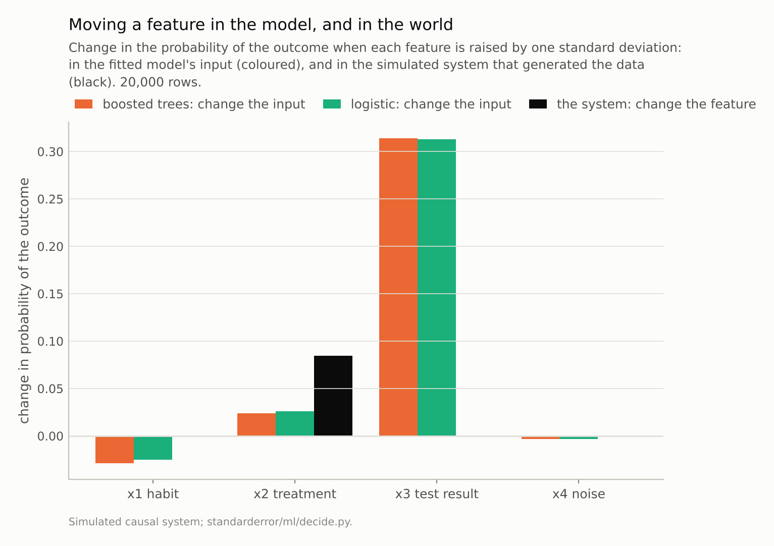
The test result moves the model’s prediction by 0.31 and the outcome by nothing; the treatment moves the outcome by 0.085 and the model by 0.024.
Three kinds of wrong
Each feature is wrong in a different way, and each way is one of the standard patterns of causal reasoning.
The test result is downstream of the outcome. It is the best predictor because it is partly a measurement of the outcome, and an intervention on it, which is like treating the thermometer, does nothing. A model that predicts well will typically lean on such variables when they are available, which is exactly what it should do as a predictor.
The habit is a fellow traveller. It is associated with lower risk only because the unmeasured trait drives both, so the model, rightly for prediction, treats it as evidence of lower risk: -0.029 per standard deviation. Encouraging the habit would not move the outcome at all.
The treatment is the one real lever, and the model nearly hides it. Its importance is 0.0021, indistinguishable from the habit’s, and the model’s what-if puts its effect at +0.024, under a third of the true +0.085. A likely reason is that the test result already records most of what the treatment did to the outcome’s underlying state, so given the test result the treatment adds little predictive information and the model has little reason to use it.
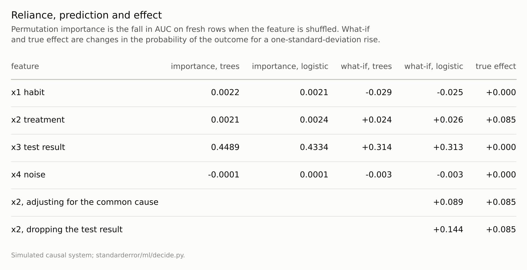
The last two rows are logistic regressions chosen with the causal structure in mind: one given the common cause, one simply without the downstream test.
What recovers the lever
The effect is recoverable from the same data, by a model built for the question rather than for prediction:
print(f"treatment alone, no other features:   {r['alone_x2']:+.3f}")
print(f"treatment, logistic on all four:      "
      f"{r['models']['logistic']['whatif']['x2 treatment']:+.3f}")
print(f"treatment, given the common cause:    {r['adjusted_x2']:+.3f}")
print(f"treatment, without the test result:   {r['without_x3_x2']:+.3f}")
print(f"treatment, true:                      "
      f"{r['true']['x2 treatment']:+.3f}")
treatment alone, no other features:   +0.202
treatment, logistic on all four:      +0.026
treatment, given the common cause:    +0.089
treatment, without the test result:   +0.144
treatment, true:                      +0.085
Given the common cause and the treatment only, a logistic regression’s what-if is +0.089, within 0.005 of the truth: adjusting for the confounder and leaving out the variable downstream of the outcome is the textbook recipe, and here it works. The naive alternative of looking at the treatment on its own is far worse: a logistic regression on the treatment alone puts its effect at +0.202, 2.4 times the truth, because people with more of the treatment also carry more of the unmeasured trait that raises the risk. The same data gave four answers for one lever, from under a third of the truth to more than twice it, depending only on which other features were in the model. Simply dropping the test result is not enough either: the habit is then only a partial stand-in for the unmeasured trait, and the treatment’s apparent effect, +0.144, overstates the truth by 70%.
The recipe needed something no predictive pipeline supplies: a measurement of the common cause, and the knowledge of which variables come before the outcome and which after. Zhao and Hastie made the conditions precise for black-box models: a partial dependence plot can be read causally when the features held fixed block every back-door path and include nothing downstream. Those conditions are about the world, and no inspection of the model can check them.
The column labelled true effect is itself what an experiment would report. It was computed by raising each feature by one standard deviation for 200,000 simulated people, everything else left to follow from the change, and comparing their outcomes with an untouched population: a randomised trial with perfect compliance, run in software. When the structure is unknown, running that trial for real, on the treatment someone actually proposes to change, is the measurement that needs no assumption about which features to include, which is why the uplift models of the next episode start from one.
Where this breaks
A system written down in advance. The causal structure here is known because it was chosen. In practice it is a hypothesis, and the adjusted estimate is only as good as the assumption that U is the only common cause.
The common cause was measurable. U was handed to the adjusted model. When it cannot be measured, adjustment is impossible, and the options are randomised experiments, instruments or bounds.
Linear effects. The treatment’s effect is linear in the log-odds. Effects that differ between people, the subject of the next episode, need more than one number.
Four features. Real models have hundreds, and the downstream ones are often hard to recognise: a variable recorded after the outcome began, or produced by the same process that records it.
What to keep
The feature the models relied on most, a consequence of the outcome, carried 0.45 of AUC and has no effect when changed.
A fellow traveller of the outcome lowered the predicted risk (-0.029) and has no effect; the real lever ranked no higher than it in importance, with a what-if under a third of its true effect.
A regression on the treatment and the common cause recovered +0.089 against a true +0.085; dropping the downstream feature alone gave +0.144.
Read importance and what-if analyses as statements about the model. Questions about what to change need the causal structure, and a model built for that question, or an experiment.
Exercise
List the features your model relies on most and, for each, write down whether it is recorded before or after the outcome could have influenced it, and what common causes it might share with the outcome.
For any feature someone proposes to change, find out whether the change has ever been made deliberately, in an experiment or a policy change, and compare what happened with what your model’s what-if predicts.
Next
When the lever is a treatment that can be given to some people and not others, the decision is whom to give it to. Episode 49 compares the usual choice, the people at highest risk, with the people the treatment would actually help.
Data
- Simulated: U standard normal (unmeasured); habit x1 = −0.8 U + 0.6 e; treatment x2 = 0.6 U + 0.8 e; outcome latent 1.2 U + 0.5 x2 + logistic noise, outcome = latent > 0; test result x3 = latent + 0.8 e; x4 pure noise. 20,000 training rows (seed 0), 20,000 fresh rows (seed 1), interventions simulated on 200,000 rows (seed 2).
- Machinery:
standarderror/ml/decide.py, tested intests/test_ml.py; scikit-learn’s HistGradientBoostingClassifier, LogisticRegression and permutation_importance (AUC, 5 repeats). - Where this stops: Pearl, Causality (2009); Hernán and Robins, Causal Inference: What If (2020); Zhao and Hastie, “Causal interpretations of black-box models”, Journal of Business & Economic Statistics (2021); episodes 16 to 18 of this series.
Reproducibility
- environment: standarderror=0.1.0, python=3.13.16, numpy=2.4.4
- code blocks: executed at build time; the values the prose quotes are pinned, so drift fails the build
- determinism: seeds 0, 1 and 2; seconds of CPU