Disclosure: this post was written with the assistance of an AI system (Claude), which wrote the analysis code, ran the experiments and drafted the text. The topic, the constraints, the data choices and the final review are the author’s.
Four base models on a simulated task, 100 to 3,000 training rows, and a logistic meta-model on their probabilities. Fitted on in-sample predictions it gave 1-NN a weight of 13 and reproduced its accuracy exactly (0.594 at 1,000 rows, against the SVM’s 0.702). Fitted on out-of-fold predictions it put its weight on the SVM and matched it (0.702), from 300 rows on never more than 0.001 above the best member; at 100 rows it scored 0.589 against 0.602. A plain average beat every member at 100 rows when no member was certain, and trailed the SVM from 300 on.
Episode 42 of Machine Learning, Taught Through What Breaks. The syllabus and the other episodes: https://jongha-jeon-dev.github.io/standarderror/lectures/
Let the data choose the weights
Episode 41 ended with an average dragged down by a member that was too weak or too sure of itself. The obvious repair is to stop weighting members equally and let the data decide how much each one counts. Wolpert called the idea stacked generalisation in 1992: fit a second model, the meta-model, whose inputs are the base models’ predictions and whose target is the label. It is now a standard ingredient of competition-winning pipelines, sold with the sentence under test: stacking learns the best way to combine models.
Four base models on episode 4’s simulated task, whose Bayes boundary is curved: logistic regression, an RBF support vector machine, a random forest and 1-nearest-neighbour. A logistic meta-model is fitted on their predicted probabilities in two ways. The quick way uses each base model’s predictions on the rows it was trained on. The careful way uses out-of-fold predictions: each training row’s prediction comes from a copy of the base model trained without it.
from standarderror.ml import combine

for r in combine.stacking_study(with_1nn=True):
    acc = r["acc"]
    print(f"{r['n']:5d} rows: SVM {acc['SVM']:.3f}, 1-NN {acc['1-NN']:.3f}"
          f" | stacks {acc['stack, in-sample']:.3f} (in-sample), "
          f"{acc['stack, out-of-fold']:.3f} (OOF)")
  100 rows: SVM 0.597, 1-NN 0.566 | stacks 0.566 (in-sample), 0.589 (OOF)
  300 rows: SVM 0.672, 1-NN 0.577 | stacks 0.577 (in-sample), 0.670 (OOF)
 1000 rows: SVM 0.702, 1-NN 0.594 | stacks 0.594 (in-sample), 0.702 (OOF)
 3000 rows: SVM 0.718, 1-NN 0.600 | stacks 0.600 (in-sample), 0.718 (OOF)
On in-sample predictions, the stack’s accuracy equals 1-NN’s at every size, to the last digit: 0.594 at 1,000 rows, the worst of the four models, while the SVM scores 0.702. On out-of-fold predictions the stack scores 0.702, the SVM’s accuracy.
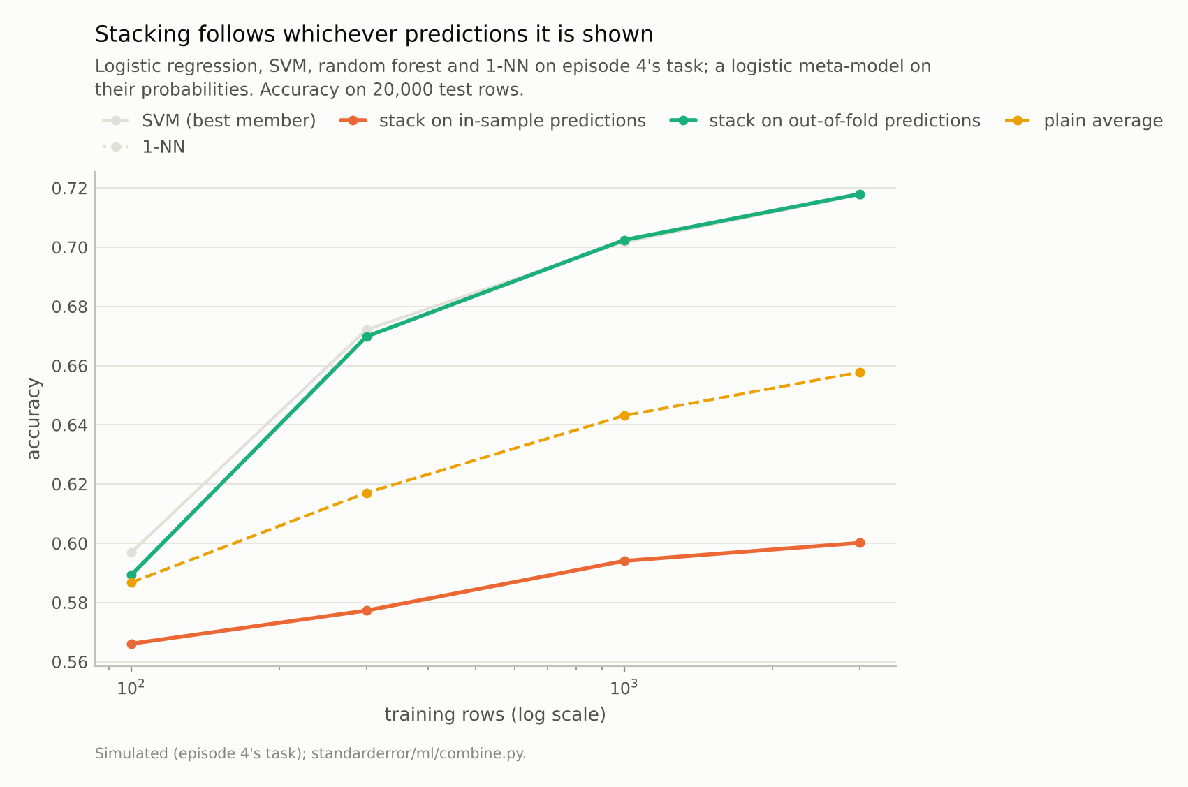
On in-sample predictions the stack became 1-NN (0.594 at 1,000 rows); on out-of-fold ones, the SVM (0.702 against 0.702).
What the meta-model trusted
The meta-model’s weights say why. On in-sample predictions, 1-NN is right about every training row, because each row is its own nearest neighbour, and the forest, whose trees are grown deep, is nearly as perfect. The meta-model sees one input that predicts the label without error and gives it a weight of +12.9, then reproduces it on test rows where it is the weakest model. Breiman made the point for regression in 1996: the level-one data must come from predictions the base models did not fit, or the combination rewards overfitting.
Replace 1-NN with 25-NN, which cannot memorise its training rows, and the same mistake picks the next best memoriser: the in-sample meta-model gives the forest a weight of +28.5, and its log loss, 1.089 at 1,000 rows, is nearly twice the SVM’s 0.570 and worse than any member’s. The meta-model is not learning which model is good; it is learning which model has seen the answers.
On out-of-fold predictions, the weights are logistic -0.24, SVM +4.56, forest +0.80, 1-NN -0.18. Almost all the weight is on the SVM, and 1-NN, whose out-of-fold predictions are as noisy as its test predictions, gets nothing.
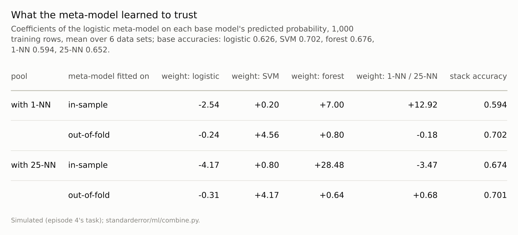
In-sample, each base model is judged on rows it has memorised to a different degree, and the meta-model rewards memory.
Honest stacking is mostly selection
Out-of-fold stacking works, in the sense that it avoids the trap. Whether it combines is another question:
for r in combine.stacking_study(with_1nn=False):   # 25-NN instead
    acc = r["acc"]
    best = r["best"]
    print(f"{r['n']:5d} rows: best member {best} {acc[best]:.3f}"
          f" | out-of-fold stack {acc['stack, out-of-fold']:.3f}, "
          f"average {acc['average']:.3f}")
  100 rows: best member forest 0.602 | out-of-fold stack 0.590, average 0.606
  300 rows: best member SVM 0.672 | out-of-fold stack 0.669, average 0.660
 1000 rows: best member SVM 0.702 | out-of-fold stack 0.701, average 0.694
 3000 rows: best member SVM 0.718 | out-of-fold stack 0.718, average 0.710
From 300 rows up, in both pools, the out-of-fold stack is within 0.0035 of the best member and never more than 0.001 above it. The meta-model has learned to pick the SVM, which a validation score would also have done. At 100 rows it is worse than the best member: 0.589, against the forest’s 0.602, though a practitioner would have had to identify the forest by validation, with its own noise. With 100 rows the out-of-fold predictions are noisy and the meta-model’s four weights are estimated from the same 100 rows, so the stack pays for estimating the combination.
The plain average shows the other side of that trade. In the pool without 1-NN, at 100 rows, it scores 0.606, above every member and 0.016 above the stack: equal weights cost nothing to estimate. From 300 rows on, logistic regression and 25-NN fall well behind the SVM, and equal weights let them drag the average below it (0.694 against 0.702 at 1,000 rows). Forecasters know this as the forecast combination puzzle: a simple average of forecasts often beats the weights estimated to combine them optimally, and Smith and Wallis traced it to the estimation error in the weights, exactly the cost visible at 100 rows here.
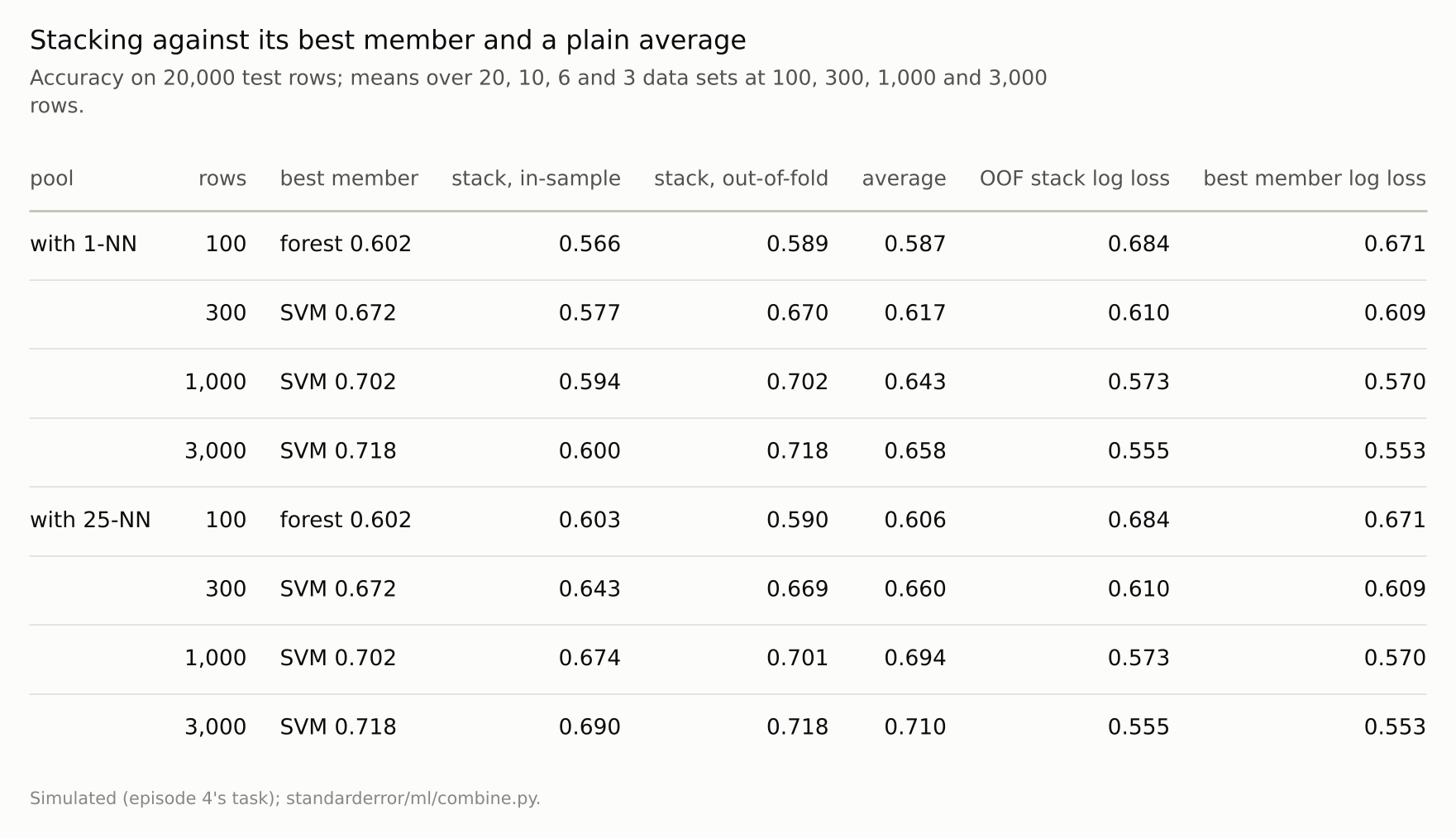
The best member is the one with the highest test accuracy at that size, which a practitioner would have to find by validation.
When stacking earns its place
Stacking improves on its best member when the members are good in different places: one model better on one region of the inputs, another elsewhere, and enough rows to learn where. On this task the SVM is best almost everywhere, so the right combination is close to “use the SVM”, and the stack found it. On tasks where diverse models of similar quality each capture part of the structure, as in many competition data sets, out-of-fold stacking can beat every member; the measurement here says what to compare it against before believing that it has.
The comparison has two baselines, not one. The stack should beat the best member chosen by validation, or it is an expensive way of choosing; and it should beat the plain average, or its weights are costing more to estimate than they gain.
Honest stacking also has a price that is easy to forget. Every base model is fitted once per fold and once more on all the rows, six fits instead of one with five folds, and the stack’s own score needs data that played no part in building it. Here that was 20,000 separate test rows. A stack scored on the same folds that produced its inputs would carry episode 35’s optimism on top of everything measured above.
Where this breaks
One task with one dominant model. The SVM’s lead from 300 rows on is large, which makes selection the right answer. With members of equal quality and complementary errors, the out-of-fold stack has more to gain and the average is harder to beat.
A linear meta-model on probabilities. Meta-models on log-odds, with non-negativity constraints on the weights (as Breiman recommended), or with the original features as extra inputs, behave differently; the in-sample trap is the same for all of them.
Few repetitions at large sizes. Three data sets at 3,000 rows; differences of a thousandth there are within noise. The in-sample stack’s exact match to 1-NN is not.
Accuracy and log loss only. A stack tuned for AUC or for a cost-weighted metric would choose differently, by the same mechanism.
What to keep
Fitted on in-sample predictions, the meta-model gave its largest weight to the model that had memorised the most: 1-NN (weight +12.9), whose accuracy it reproduced exactly, or the forest when 1-NN was absent.
Fitted on out-of-fold predictions it chose the SVM and matched it to within 0.0035 from 300 rows on, never more than 0.001 above it; at 100 rows it lost 0.013 to the best member.
A plain average beat every member at 100 rows when no member was certain, and trailed the best member once the weak ones fell behind.
Fit stacks on out-of-fold predictions only, and keep a stack only if it beats both the best single model and the plain average on data neither has seen.
Exercise
Take a stacked model and print the meta-model’s weights. Refit the meta-model on in-sample base predictions instead of out-of-fold ones and print them again.
Then score three things on a held-out set: the stack, the base model with the best validation score, and a plain average of the base models. If the stack’s weights are concentrated on one model, compare it with that model alone; if it is not better than the average, its weights are not worth their estimation error.
Next
Stacking and averaging both end in the same question: is this model better than that one? Episode 43 looks at a combination inside a single model, naive Bayes adding up evidence feature by feature, before episode 44 turns to the tests that compare models.
Data
- Simulated: episode 4’s two-class Gaussian task in 10 dimensions, Bayes error 0.268; training sets of 100, 300, 1,000 and 3,000 rows (20, 10, 6 and 3 data sets, seeds from 0); 20,000 fixed test rows.
- Machinery:
standarderror/ml/combine.py, tested intests/test_ml.py; scikit-learn’s LogisticRegression, SVC (RBF, Platt probabilities), RandomForestClassifier (200 trees), KNeighborsClassifier (k = 1 or 25); meta-model LogisticRegression (C = 10,000) on the base probabilities; out-of-fold predictions from five stratified folds. - Where this stops: Wolpert, “Stacked generalization”, Neural Networks (1992); Breiman, “Stacked regressions”, Machine Learning (1996); Smith and Wallis, “A simple explanation of the forecast combination puzzle”, Oxford Bulletin of Economics and Statistics (2009).
Reproducibility
- environment: standarderror=0.1.0, python=3.13.16, numpy=2.4.4
- code blocks: executed at build time; the values the prose quotes are pinned, so drift fails the build
- determinism: data seeds from 0, fold shuffles from the data seed, model random_state 0; about six minutes of CPU