Disclosure: this post was written with the assistance of an AI system (Claude), which wrote the analysis code, ran the experiments and drafted the text. The topic, the constraints, the data choices and the final review are the author’s.
Six classifiers on the digits, and the averaged probabilities of all 57 combinations of two or more. 11 combinations beat their best member’s accuracy and 8 fell below their members’ mean. Averaged with a single decision tree, whose probabilities are all 0 or 1, an SVM scoring 0.977 lost every disagreement and the average scored the tree’s 0.825. The guarantee that does hold is weaker: the average’s log loss was at or below the members’ mean every time, and on diabetes the average of four regressors improved on their mean error by exactly their spread, 576, and still lost to ridge regression alone.
Episode 41 of Machine Learning, Taught Through What Breaks. The syllabus and the other episodes: https://jongha-jeon-dev.github.io/standarderror/lectures/
The free lunch
Forty episodes measured single models and the data under them. Arc IX turns to what is done with several models: combining them, stacking them, and deciding which is better. The most common combination is the simplest. Train a few different models, average their predicted probabilities, and report the average, on the strength of a sentence that sounds like a theorem: averaging several models gives a better model than any of them.
Six classifiers were trained on half the digits and scored on the other half, five times: regularised logistic regression, a support vector machine, five-nearest-neighbours, a random forest, Gaussian naive Bayes and a single decision tree. Their accuracies range from 0.825 for the tree to 0.981 for nearest neighbours. Every combination of two or more, 57 in all, was averaged.
from standarderror.ml import combine

t = combine.averaging_table()   # 57 combinations, 5 half-splits
best = sum(r["acc"] > r["best_acc"] for r in t)
below = sum(r["acc"] < r["mean_acc"] for r in t)
print(f"beat their best member: {best} of {len(t)}")
print(f"below their members' mean accuracy: {below} of {len(t)}")
top = max(t, key=lambda r: r["acc"])
print(f"best combination: {' + '.join(top['members'])}, "
      f"{top['acc']:.4f} against its best member's {top['best_acc']:.4f}")
beat their best member: 11 of 57
below their members' mean accuracy: 8 of 57
best combination: SVM + 5-NN + forest, 0.9873 against its best member's 0.9813
Only 11 of the 57 averages beat the best model in them. The best average, of the SVM, nearest neighbours and the forest, gained 0.0060 over nearest neighbours alone, about half a point. And 8 averages did worse than the mean of their members, which an average is supposed to beat by construction.
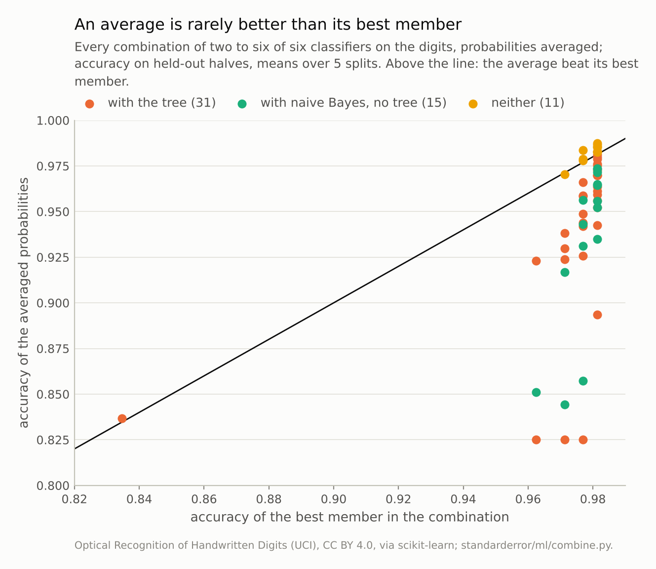
One of the 31 combinations containing the decision tree beat its best member, pairing it with naive Bayes; 11 of 57 combinations did.
Averaging is not voting
The worst averages contain the decision tree, and the worst of those are pairs. Averaged with logistic regression, the SVM or the forest, the tree’s accuracy, 0.825, is exactly what the pair scored. The reason is in what a single fully grown tree predicts: each leaf holds one class, so its predicted probability is 1 for one digit and 0 for the rest, on 100% of the digits, while those three models are almost never that certain about anything (the forest on 0.3% of digits).
p = combine.averaging_pair("SVM", "tree")
print(f"SVM + tree: accuracy {p['acc']:.4f}")
print(f"on {p['disagree']} disagreements the average sided with "
      f"the tree {p['with_b']:.0%} of the time")
SVM + tree: accuracy 0.8251
on 819 disagreements the average sided with the tree 100% of the time
Average a probability of 1 with one other model’s probabilities and the result is at least one half for the tree’s class, which no other class can beat unless the other model is just as certain. On all 819 digits where the SVM and the tree disagreed, the average sided with the tree. In larger averages the tree’s certain class is guaranteed only a share of one over the number of members, and confident agreement among the others can outweigh it, so the averages recover, but only one of the 31 combinations containing the tree beat its best member: the tree with naive Bayes, the two weakest models of the six. The average weights each member by its confidence, and the tree’s confidence is unconditional. Naive Bayes, certain about 52% of digits, does the same to a lesser degree: averaged with the SVM it won 86% of their disagreements, and the pair scored 0.857.
Calibrating the tree first removes the certainty: an isotonic recalibration by internal cross-validation leaves it certain about no digit, and the SVM-plus-tree average rises to 0.973. That is far better, and still below the SVM alone (0.977): the tree is a weaker model, and averaging with a weaker model is a cost unless it is wrong on different digits from the stronger one.
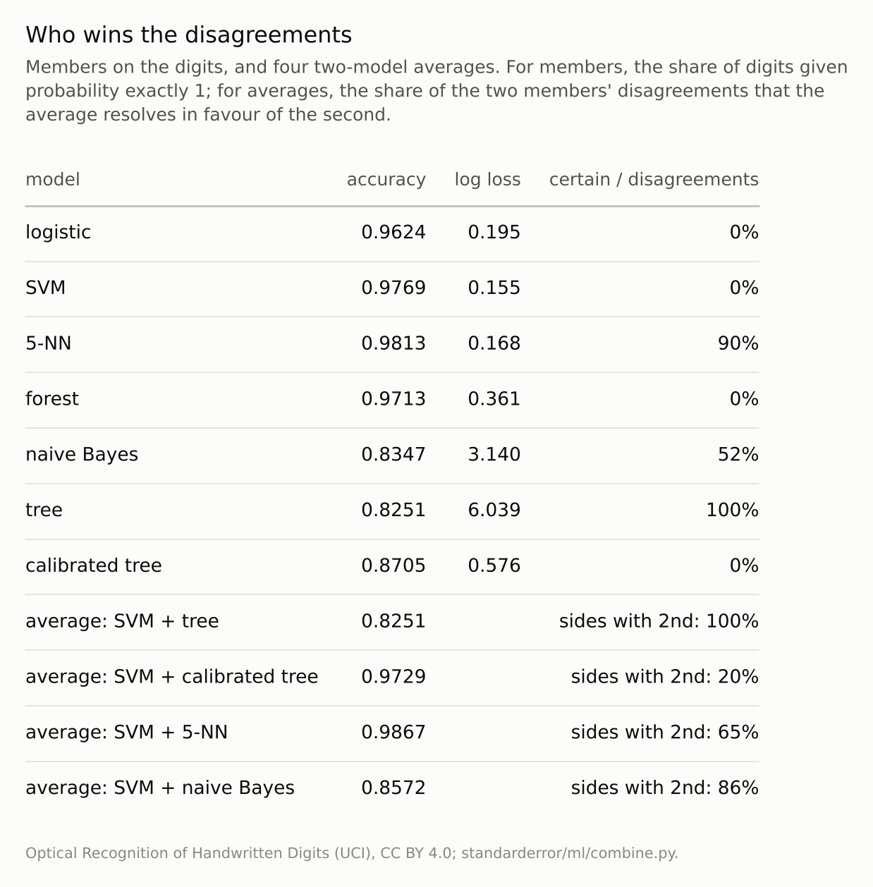
The tree is certain about every digit, so paired with a model that is almost never certain it wins every disagreement. Calibrating it removes that, but the pair still trails the SVM alone.
What is guaranteed
There is a real theorem behind the sentence, and it says less. For squared error, Krogh and Vedelsby showed in 1995 that the error of an equally weighted average is exactly the members’ mean error minus their spread around the average, which they called the ambiguity. Since the spread cannot be negative, the average is never worse than the average member, and it improves on the average member by as much as the members disagree. On the diabetes data, with four regressors:
a = combine.ambiguity()          # diabetes, four regressors
print(f"mean member {a['mean_member']:.1f} - spread "
      f"{a['ambiguity']:.1f} = average {a['ensemble']:.1f} "
      f"(gap {a['identity_gap']:.0e})")
print("members: " + ", ".join(f"{k} {v:.0f}"
                              for k, v in a["members"].items()))
mean member 4018.6 - spread 576.3 = average 3442.4 (gap 9e-13)
members: ridge 3041, 10-NN 3152, forest 3552, tree 6329
The identity holds to twelve decimal places. The average improves on the mean member by 576, all of it the members’ disagreement. And it is still worse than ridge regression alone, 3041 against 3442: the single tree’s error was so large that the mean member started far behind the best one, and the spread did not close the gap.
The same kind of guarantee holds for log loss, because log loss is convex in the probabilities: the averaged probabilities’ log loss was at or below the members’ mean in all 57 combinations. It was below the best member’s in 13. Neither guarantee mentions the best member, and accuracy, which is not convex, has no such guarantee at all; that is how 8 combinations fell below even their members’ mean.
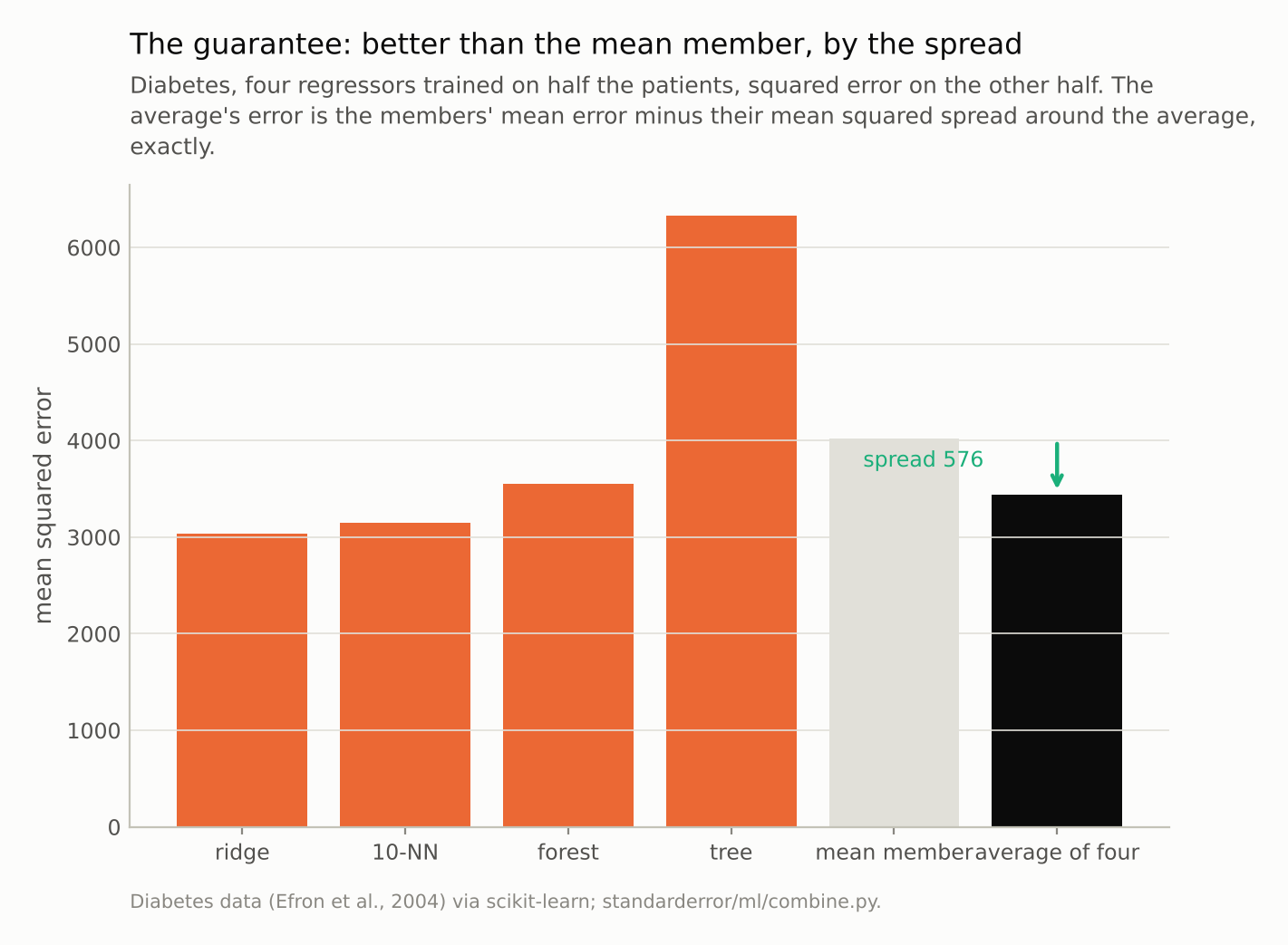
4019 − 576 = 3442, to within 9e-13; ridge alone scored 3041.
When averaging pays
The combinations that did beat their best member share two properties: their members are of similar quality, and they are wrong on different digits. The SVM and nearest neighbours, 0.977 and 0.981 alone, disagreed on 123 digits across the five splits and averaged to 0.9867, better than either. Dietterich’s account of why ensembles work rests on exactly these two conditions, accuracy and diversity, and random forests are built to meet them: many trees of equal quality, made different on purpose.
So the useful version of the sentence is conditional. An average of models that are about equally good and differently wrong is usually better than each of them; an average that includes a much weaker or a much more confident model is usually worse than the best. Calibrating the members first stops confidence from deciding the vote, and weighting them by validated performance stops a weak model from diluting a strong one, which is where episode 42 picks up.
Where this breaks
One data set where a single model is excellent. Nearest neighbours alone scores 0.98 on the digits, which leaves little room for any combination to gain. Harder tasks with more balanced members may leave more room; that was not measured here.
Unweighted averages. Every member counted equally. Weighted averages and stacking are the obvious refinements, and their own failure modes are the next episode.
A deliberately bad member. A fully grown single tree is not something anyone would put in an ensemble on purpose; it is here because its certainty makes the mechanism visible. Any overconfident member, such as an unregularised boosted model late in training, does the same in a milder form.
Five splits. The counts of combinations above and below their best member come from one set of five half splits and could shift with others; the tree’s capture of every pair it joined with a less certain model follows from its probabilities and would not.
What to keep
Of 57 averaged combinations of six classifiers on the digits, 11 beat their best member and 8 fell below their members’ mean accuracy.
Averaging probabilities weights each model by its confidence. A tree certain about every digit won all 819 disagreements with the SVM, the pair scored 0.825, and only one of the 31 combinations containing the tree, the one pairing it with naive Bayes, beat its best member.
The guarantee is against the mean member: for squared error, the average’s error is the mean member’s minus their spread, exactly; on diabetes that still left it behind ridge regression alone.
Average models of similar quality that make different mistakes, calibrate them first, and compare the average with the best single model before adopting it.
Exercise
Take an ensemble you use and score each member alone on held-out data, alongside the ensemble. Then compute, for every pair of members, the share of rows on which they disagree, and the share of predictions each makes with probability above 0.99.
If the ensemble is not better than its best member, look for a member that is much weaker or much more confident than the rest, and rescore the ensemble without it.
Next
The natural fix for a bad member is to let the data choose the weights. Episode 42 fits those weights with a second model, stacking, and measures what it learns from in-sample predictions, from out-of-fold ones, and how often it beats picking the best member.
Data
- Optical Recognition of Handwritten Digits (UCI), as bundled with scikit-learn, CC BY 4.0; 1,797 images, five stratified half splits (seeds 0 to 4).
- Diabetes data of Efron et al. (2004), as bundled with scikit-learn; one half split (seed 0).
- Machinery:
standarderror/ml/combine.py, tested intests/test_ml.py; scikit-learn’s LogisticRegression (C = 0.1), SVC (RBF, Platt probabilities), KNeighborsClassifier (k = 5), RandomForestClassifier (300 trees), GaussianNB, DecisionTreeClassifier, CalibratedClassifierCV (isotonic, five folds); RidgeCV, KNeighborsRegressor (k = 10), RandomForestRegressor, DecisionTreeRegressor. - Where this stops: Krogh and Vedelsby, “Neural network ensembles, cross validation, and active learning”, NeurIPS (1995); Dietterich, “Ensemble methods in machine learning” (2000); Kuncheva, Combining Pattern Classifiers (2004).
Reproducibility
- environment: standarderror=0.1.0, python=3.13.16, numpy=2.4.4
- code blocks: executed at build time; the values the prose quotes are pinned, so drift fails the build
- determinism: split seeds 0 to 4 (digits) and 0 (diabetes); model random_state 0; under a minute of CPU