Disclosure: this post was written with the assistance of an AI system (Claude), which wrote the analysis code, ran the experiments and drafted the text. The topic, the constraints, the data choices and the final review are the author’s.
2,000 simulated rows from 2,000, 400, 100, 40 or 20 subjects, each subject with a feature signature and an outcome propensity that do not carry over. With 2,000 subjects, row-level and subject-level cross-validation matched accuracy on new people to within a point. With 20 subjects, row-level cross-validation scored five-nearest-neighbours at 0.825 against 0.685 on new people, and a forest at 0.847 against 0.770; subject-level folds gave 0.662 and 0.751. 6,400 rows from 20 subjects trained a logistic model to 0.788, about what 100 rows from 100 subjects gave.
Episode 37 of Machine Learning, Taught Through What Breaks. The syllabus and the other episodes: https://jongha-jeon-dev.github.io/standarderror/lectures/
Twenty people, a hundred rows each
Episode 36 found that rows close in time are a problem only when they share something the model cannot see. People are the other common source of rows that share something: a patient measured at every visit, a customer with a year of transactions, a speaker with a hundred recordings, a writer with a page of digits. Episode 3 measured exact duplicates straddling folds and noted that near-duplicates, such as the same patient twice, leak by the same mechanism with less force. This episode measures that case, and the sentence that makes it easy to miss: more rows means more data, and cross-validation over the rows measures how the model will do.
The simulation gives each subject two things that belong to them alone. One is a signature: an offset added to all ten of their features, so their rows sit together in feature space. The other is a propensity: an offset added to the log-odds of all their outcomes, so some people are simply more often positive than others. Neither tells you anything about a new person. What does carry over is a relationship between two features and the outcome, the same for everyone. Each design has 2,000 rows; what changes is how many people they come from.
from standarderror.ml import rows

for r in rows.subject_cv():   # 2,000 rows each time
    if r["model"] == "5-NN":
        print(f"{r['subjects']:5d} subjects x {r['per']:3d} rows: "
              f"row CV {r['row']:.3f}, subject CV {r['subject']:.3f}, "
              f"new people {r['new']:.3f}")
 2000 subjects x   1 rows: row CV 0.737, subject CV 0.741, new people 0.741
  400 subjects x   5 rows: row CV 0.782, subject CV 0.747, new people 0.735
  100 subjects x  20 rows: row CV 0.827, subject CV 0.719, new people 0.718
   40 subjects x  50 rows: row CV 0.818, subject CV 0.674, new people 0.704
   20 subjects x 100 rows: row CV 0.825, subject CV 0.662, new people 0.685
With one row from each of 2,000 people, row-level cross-validation and the truth agree: 0.737 against 0.741. As the same 2,000 rows come from fewer people, the two move in opposite directions. Row-level cross-validation rises, to above 0.81 from 100 people down and 0.825 with 20, while accuracy on new people falls at every step, to 0.685. Read through row-level folds, the data sets built from 100 people or fewer look like the best of the five, and the one from 20 people scores the forest highest of all.
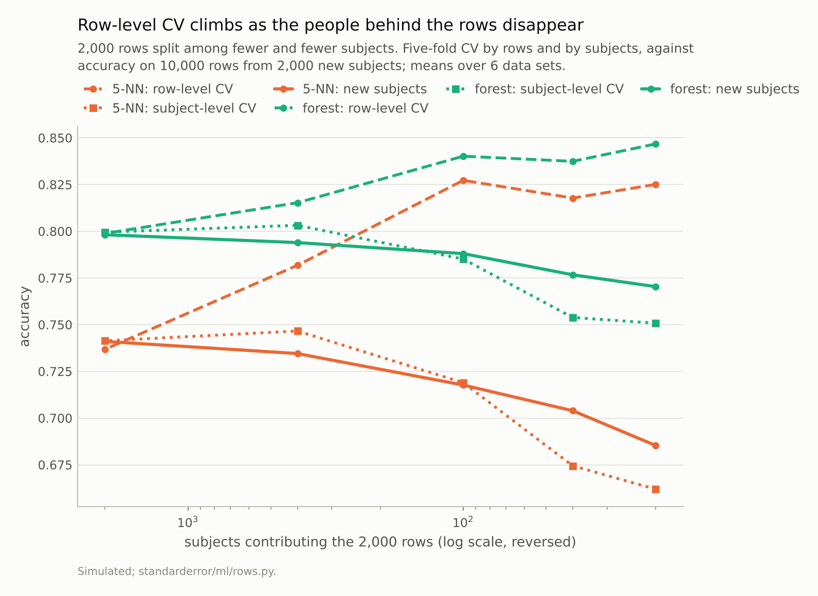
From 20 subjects, row-level CV scored five-nearest-neighbours at 0.825; on new people it scored 0.685.
What the folds were measuring
A row-level fold holds out one-fifth of each person’s rows and trains on the other four-fifths. A held-out row’s nearest neighbours in feature space are almost all rows from the same person: with 20 people, 96.6% of the five nearest training rows, because the signature puts them together, and those rows carry the same propensity. Five-nearest-neighbours answers by asking the person’s other rows what usually happens to this person, which is an excellent way to predict a person it has already met and no way at all to predict a new one.
The forest finds the same shortcut through its splits: 0.847 under row-level folds, 0.770 on new people. Logistic regression, which can only draw one plane through the feature space, has less room to memorise people, and its gap is smaller but not zero: 0.824 against 0.783. A plausible reason, not isolated here, is that with 20 people a few of them can by chance have signatures that line up with their propensities, and a linear model fits that accident too.
The repair is to make the folds match the question. Subject-level cross-validation keeps every person’s rows in a single fold, so each held-out row belongs to someone the model has never seen. It scored the nearest-neighbour model at 0.662 and the forest at 0.751, slightly below the truth, likely in part because each fold trains on 16 people instead of 20. That pessimism is a feature of very few groups: with 400 subjects the same folds were a little optimistic, by up to 0.012.
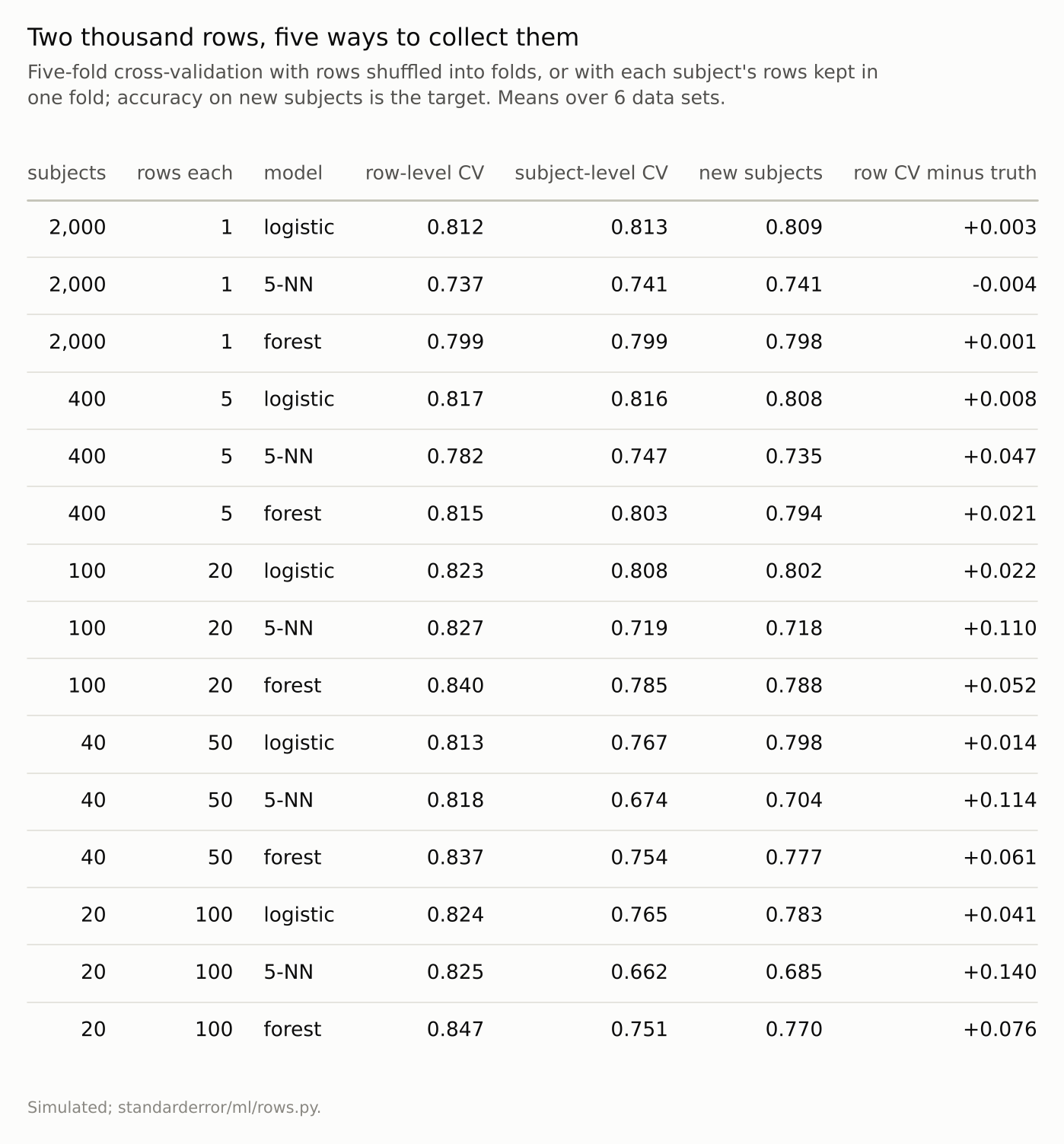
Row-level cross-validation measures how well the model knows the people it has met. Subject-level cross-validation measures how well it does on new ones.
What more rows buy
The second half of the sentence, that more rows mean more data, is measured directly by growing the training set two ways: one row from each of N new people, or N/20 rows from each of the same 20 people.
for r in rows.subject_growth():
    print(f"{r['rows']:5d} rows, {r['how']:12s}: logistic "
          f"{r['logistic']:.3f}, forest {r['forest']:.3f}")
  100 rows, new subjects: logistic 0.785, forest 0.752
  100 rows, 20 subjects : logistic 0.772, forest 0.731
  400 rows, new subjects: logistic 0.804, forest 0.783
  400 rows, 20 subjects : logistic 0.782, forest 0.751
 1600 rows, new subjects: logistic 0.809, forest 0.796
 1600 rows, 20 subjects : logistic 0.787, forest 0.766
 6400 rows, new subjects: logistic 0.810, forest 0.798
 6400 rows, 20 subjects : logistic 0.788, forest 0.777
One row per person keeps improving: logistic regression goes from 0.785 at 100 rows to 0.810 at 6,400. Twenty people with more and more rows each barely move: from 0.772 to 0.788, about what 100 rows from 100 people gave (0.785) and below what 400 rows from 400 people gave (0.804). For the forest, 6,400 rows from 20 people reached 0.777, again below 400 rows from 400 people (0.783).
Survey statisticians have a name for this: the design effect. Kish’s formula says that m rows from each cluster, with intra-cluster correlation ρ, are worth n / (1 + (m − 1)ρ) independent rows. When the thing that varies between people is large compared with what varies within them, as it is here, extra rows from the same person add almost nothing about what is true of people in general. They add a great deal about that person, which is what row-level folds reward.
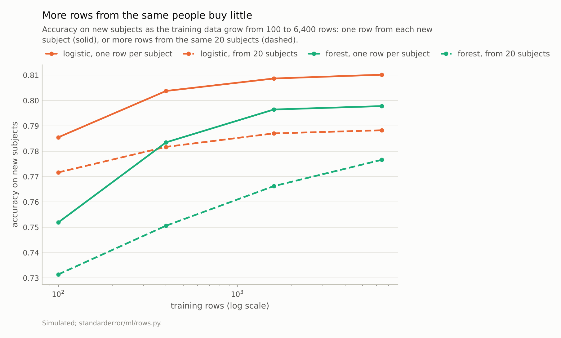
6,400 rows from 20 subjects: logistic regression 0.788. 400 rows from 400 subjects: 0.804.
Which question is being asked
Row-level cross-validation is not wrong in itself; it answers a different question. If the model will only ever be used on the people it was trained on, such as predicting a known customer’s next purchase or a known patient’s next reading, then rows from the same person are exactly the relevant test, and subject-level folds would be too pessimistic. Saeb and colleagues made the point for clinical models built from smartphone data: the right split is the one that imitates the use. The mistake is to answer one question and report the answer to the other.
The same logic covers any grouping the deployment will not share: hospitals when a model moves to a new hospital, schools, devices, plots of land in ecology, and the writers of handwritten digits. Roberts and colleagues reviewed it for temporal, spatial and phylogenetic groupings and reached the same rule: block the folds by whatever the new data will be new in.
Where this breaks
Strong subject effects, by construction. The signature and the propensity both have a standard deviation of 2, large enough that a person’s rows are easy to recognise. Where between-person differences are small, the gap between the two kinds of cross-validation shrinks towards the one-row-per-person case, where it vanishes.
Effects that do not transfer at all. Here nothing about a person helps with a new one. In practice some person-level traits are measured, and a model that uses them generalises better; the problem is the part that is not measured.
Twenty subjects is few. Subject-level cross-validation with 20 groups trains on 16 of them per fold and its estimates are noisy from data set to data set. With very few subjects, leave-one-subject-out folds and an honest statement of the uncertainty are the best available.
Balanced subjects. Every subject contributed the same number of rows. With a few heavy contributors, row-level scores are dominated by them, and the distortion can be worse.
What to keep
Rows from the same person share what makes that person different. With 2,000 rows from 20 people, row-level cross-validation scored five-nearest-neighbours at 0.825; on new people it scored 0.685.
As the same rows came from fewer people, row-level scores went up, from 0.737 to above 0.81, while true accuracy fell at every step, so row-level folds favoured exactly the data sets that generalise worst.
With 20 subjects, subject-level folds matched the truth to within 0.023, slightly pessimistic.
6,400 rows from 20 people trained logistic regression to 0.788, about what 100 rows from 100 people gave. Count people, not rows, and split the folds by whatever the deployment will be new in.
Exercise
For a data set with an identifier for the source of each row (person, account, device, site), count the rows per identifier and compute the intra-class correlation of your target within identifiers.
Then cross-validate your model twice, once with shuffled rows and once with folds grouped by the identifier. The difference between the two scores is how much of your model’s apparent skill is recognising sources it has already seen; plug the correlation into Kish’s formula to see how many independent rows you really have.
Next
Time and people decide which rows resemble each other. Episode 38 turns to rows that are incomplete, and asks whether a missing value is noise to be filled in or information the process that produced the data left behind.
Data
- Simulated: each subject has a signature in ten features (normal, sd 2) added to every one of its rows, and a propensity (normal, sd 2) added to every row’s log-odds; the part of the outcome that carries over to new subjects is 1.5 x_1 + x_2. Six data sets per design (seeds 0 to 5); new subjects: 2,000 of them with 5 rows each (seeds 1,000 to 1,005).
- Machinery:
standarderror/ml/rows.py, tested intests/test_ml.py; scikit-learn’s LogisticRegression, KNeighborsClassifier (k = 5), RandomForestClassifier (50 trees), KFold with shuffling and GroupKFold, five folds each. - Where this stops: Kish, Survey Sampling (1965) on the design effect; Saeb et al., “The need to approximate the use-case in clinical machine learning”, GigaScience (2017); Roberts et al., Ecography (2017); episode 3 of this series.
Reproducibility
- environment: standarderror=0.1.0, python=3.13.16, numpy=2.4.4
- code blocks: executed at build time; the values the prose quotes are pinned, so drift fails the build
- determinism: seeds as listed; shuffled folds from the data set’s seed; about two minutes of CPU