Disclosure: this post was written with the assistance of an AI system (Claude), which wrote the analysis code, ran the experiments and drafted the text. The topic, the constraints, the data choices and the final review are the author’s.
For uniform points, the nearest neighbour’s distance over the median distance rose from 0.03 in two dimensions to 0.94 in 1,024: in high dimensions the nearest point is barely nearer than the rest. The 1,797 digits have 64 pixels and a ratio of 0.34, the value uniform data have in about 8 dimensions, and five-nearest-neighbours scores 0.986 on them. Appending 1,024 uniform noise columns raised the ratio to 0.94 and dropped nearest neighbours to 0.659, while logistic regression fell from 0.969 to 0.871.
Episode 33 of Machine Learning, Taught Through What Breaks. The syllabus and the other episodes: https://jongha-jeon-dev.github.io/standarderror/lectures/
The nearest of many equals
Episode 32 clustered by distance and found that the clusters depended on what distance could see. Nearest-neighbour methods depend on distance even more directly: to classify a point, find the training points closest to it and take their vote. The textbook warning attached to them is the curse of dimensionality, usually stated as the sentence under test: in high dimensions, nearest neighbours stop meaning anything.
The warning has a precise form. Beyer and colleagues showed that for many distributions, as the number of dimensions grows, the distance to the nearest point and the distance to the farthest become nearly equal, so “nearest” no longer singles anything out. For points spread uniformly over a cube it is easy to see:
from standarderror.ml import around

for r in around.contrast():          # 1,000 uniform points per d
    print(f"d = {r['d']:5d}: nearest / median distance {r['ratio']:.3f}, "
          f"(farthest - nearest) / nearest {r['spread']:.2f}")
d =     1: nearest / median distance 0.001, (farthest - nearest) / nearest 2011.69
d =     2: nearest / median distance 0.028, (farthest - nearest) / nearest 70.79
d =     4: nearest / median distance 0.144, (farthest - nearest) / nearest 11.06
d =     8: nearest / median distance 0.339, (farthest - nearest) / nearest 3.55
d =    16: nearest / median distance 0.526, (farthest - nearest) / nearest 1.66
d =    64: nearest / median distance 0.774, (farthest - nearest) / nearest 0.56
d =   256: nearest / median distance 0.886, (farthest - nearest) / nearest 0.25
d =  1024: nearest / median distance 0.944, (farthest - nearest) / nearest 0.12
In two dimensions the nearest of 1,000 points is at 0.03 of the median distance, and the farthest is 71 times farther than the nearest. In 1,024 dimensions the nearest is at 0.94 of the median, and the farthest only 12% farther. Every point is about equally far from every other. A vote among the “nearest” five is a vote among five points chosen almost at random.
So the sentence is true of uniform points. The question is whether it is true of data.
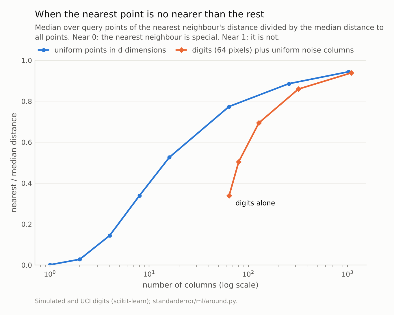
The digits’ 64 pixels have the ratio uniform data have in about 8 dimensions. Noise columns move them up the curve.
Sixty-four pixels, eight dimensions
The digits are 8 × 8 images, 64 numbers each: by the column count, a high-dimensional data set. Here is the same ratio for them, and what happens when uniform noise columns are appended to each image:
for r in around.neighbours_noise():  # digits plus uniform noise columns
    print(f"{r['d']:5d} columns: nearest / median {r['ratio']:.3f}, "
          f"5-NN {r['knn']:.3f}, logistic {r['logistic']:.3f}")
   64 columns: nearest / median 0.339, 5-NN 0.986, logistic 0.969
   80 columns: nearest / median 0.504, 5-NN 0.981, logistic 0.960
  128 columns: nearest / median 0.695, 5-NN 0.960, logistic 0.950
  320 columns: nearest / median 0.859, 5-NN 0.867, logistic 0.924
 1088 columns: nearest / median 0.938, 5-NN 0.659, logistic 0.871
On the digits alone the nearest image is at 0.34 of the median distance. Uniform points reach that ratio at about 8 dimensions, not 64. And five-nearest-neighbours, the method the curse is supposed to defeat, scores 0.986, higher than logistic regression’s 0.969.
The reason is that the 64 pixels are not 64 independent directions. Strokes are continuous, so neighbouring pixels move together; most of the 8 × 8 grid is blank for most digits; and the images of one digit vary in a few ways (slant, thickness, size) rather than in 64. The points occupy a thin, curved region of the 64-dimensional cube, and distances within that region behave like distances in a much smaller space. Levina and Bickel call the dimension of that region the intrinsic dimension and estimate it from exactly this kind of nearest-neighbour statistic.
The other measure agrees. The gap between a digit’s farthest and nearest neighbours, as a multiple of the nearest distance, is 3.0; for uniform points it is 3.6 in 8 dimensions and 0.56 in 64. By either measure the digits look like a space of a handful of dimensions, not of sixty-four.
What matters for the curse, then, is not how many columns the data have but how many directions they actually spread in.
What breaks it: columns that carry nothing
The noise columns show where the curse does bite. Each added column is uniform on the same 0-to-1 scale as the pixels and unrelated to the digit. Sixteen of them barely matter. With 256, the ratio is 0.86 and nearest neighbours fall to 0.867. With 1,024, the ratio is 0.94, about what 1,024 uniform dimensions give, and nearest neighbours score 0.659.
The noise columns fill their dimensions, which the pixels do not, and Euclidean distance weighs every column equally. Once the noise columns outnumber the pixels sixteen to one, the distance between two images is mostly the distance between their noise, and the nearest neighbours are nearest in noise.
Logistic regression suffers far less, falling from 0.969 to 0.871. It learns a weight for every column and can give the noise columns weights near zero, which a plain distance cannot. The drop for nearest neighbours is 3.3 times the drop for logistic regression. The practical curse is therefore a curse on methods that treat every column as equally informative, in data with many uninformative columns.
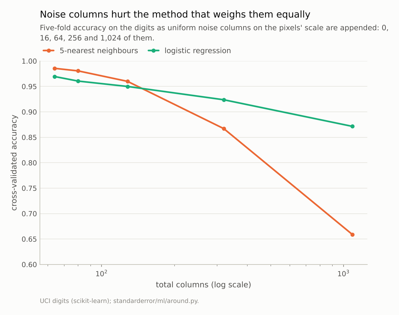
With 1,024 noise columns nearest neighbours score 0.659 and logistic regression 0.871.
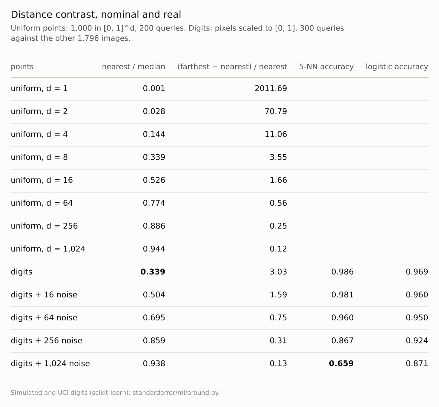
The digits sit between uniform data in 4 and 16 dimensions. The noise columns carry them to where 1,024 uniform dimensions are.
The repair is to stop counting the noise
If the trouble is columns that carry nothing, the repair is to stop letting them into the distance. The bluntest version keeps the 64 columns whose values differ most between digit classes, by an analysis-of-variance F statistic, chosen inside each training fold so the test images play no part in the choice:
r = around.neighbours_repair()   # 1,024 noise columns, keep 64 by F
print(f"5-NN on the {r['keep']} selected columns: {r['knn']:.3f}; "
      f"real pixels among them: {r['real_share']:.0%}")
5-NN on the 64 selected columns: 0.982; real pixels among them: 88%
With the 1,024 noise columns still present in the data, nearest neighbours on the 64 kept columns score 0.982, against 0.659 without selection and 0.986 on the clean digits. The selection is not perfect: 88% of the columns it keeps are real pixels, and the rest are noise columns that happened to differ between classes by chance. It is enough. Distance is useful again as soon as most of it is computed on columns that carry information.
That is also the honest reading of the curse. It is not a property of a number of columns, which a selection step can change without changing the problem. It is a property of how the information in the data is spread across them. Many columns, few of them informative, is the hard case. Many columns, all of them moving together with the thing being predicted, is the easy one, and the digits are much closer to it.
Where this breaks
Uniform noise is the worst kind. Real irrelevant features are often correlated with each other or nearly constant, and fill fewer dimensions than independent uniform columns; they hurt less.
Euclidean distance, unweighted. Scaling or selecting features, learning a metric, or using a representation from a trained model all change what “near” means, and are the standard repairs. None was applied here, by design.
One data set with low intrinsic dimension. Data that genuinely spread in many directions, such as some text or genomic data, can be nearly as hard as the uniform case. The point is that the column count does not tell you which case you are in; the distance ratio, or an intrinsic-dimension estimate, does.
k = 5, one split scheme. Other choices of k move the numbers a little and not the pattern.
What to keep
For points that fill their space, distances concentrate: the nearest/median ratio rose from 0.03 in 2 uniform dimensions to 0.94 in 1,024.
Real data rarely fill their columns. The digits’ 64 pixels had the ratio of about 8 uniform dimensions, and five-nearest-neighbours scored 0.986.
Irrelevant columns do fill their dimensions. With 1,024 noise columns nearest neighbours fell to 0.659; logistic regression, which weights columns, fell to 0.871.
Before blaming dimension, measure the nearest/median distance ratio of your data, and remove or down-weight columns that carry nothing.
Exercise
For a data set you use with a distance-based method, take 200 rows and compute, for each, its nearest distance over its median distance to the rest. Then compute the same for uniform data with your number of columns, and with a few smaller numbers.
Find the uniform dimension that matches your data’s ratio. If it is far below your column count, the curse is not your problem; if it is close, check how many of your columns actually carry information about the target.
Next
Distances decide which neighbours vote; probabilities decide how much a prediction should be trusted. Episode 34 measures the standard repair for untrustworthy probabilities, recalibration, and asks how much data it needs and what kind of trust it buys.
Data
- Simulated: 1,000 points and 200 queries uniform on [0, 1]^d for d from 1 to 1,024; seed 0.
- Optical Recognition of Handwritten Digits (UCI), as bundled with scikit-learn, CC BY 4.0; pixels divided by 16, with 0 to 1,024 uniform [0, 1] columns appended (seed 0).
- Machinery:
standarderror/ml/around.py, tested intests/test_ml.py; Euclidean distances, scikit-learn’s KNeighborsClassifier (k = 5) and LogisticRegression, five-fold stratified cross-validation. - Where this stops: Beyer, Goldstein, Ramakrishnan and Shaft, “When is ’nearest neighbor’ meaningful?”, ICDT (1999); Levina and Bickel, “Maximum likelihood estimation of intrinsic dimension”, NeurIPS (2004).
Reproducibility
- environment: standarderror=0.1.0, python=3.13.16, numpy=2.4.4
- code blocks: executed at build time; the values the prose quotes are pinned, so drift fails the build
- determinism: uniform points and noise columns from seed 0; shuffled folds with random_state 0