Disclosure: this post was written with the assistance of an AI system (Claude), which wrote the analysis code, ran the experiments and drafted the text. The topic, the constraints, the data choices and the final review are the author’s.
A two-layer network with batch normalisation scored 0.990 on 100 test digits in inference mode. In training mode, each digit’s label changed with its random batch companions in 45% of batches of 2, 20% of batches of 4, 3.2% of batches of 16 and 0.6% of batches of 64; with 15 companions from one class, in 23%. Trained in batches of 2, the normalised network scored 0.863 in inference mode against 0.972 without normalisation; trained in batches of 16 or 64 it scored 0.5 and 0.8 points higher, over three seeds.
Episode 24 of Machine Learning, Taught Through What Breaks. The syllabus and the other episodes: https://jongha-jeon-dev.github.io/standarderror/lectures/
A layer with two modes
Episode 23 compared optimisers on networks with nothing between their layers but activations. Most modern networks have something else there: a normalisation layer. Batch normalisation, the first to be widely used, takes each unit’s values across the examples in a minibatch, subtracts their mean, divides by their standard deviation, and then applies a learned scale and shift. Training is faster and less sensitive to the initial scale, which is the problem episode 21 measured.
The usual description is the sentence under test: batch normalisation normalises each example, rescaling its activations to a standard range. The mean and standard deviation, though, are not the example’s. They are the batch’s. During training, an example’s output is computed from statistics of the other examples it happens to be batched with. At inference, the layer switches to running averages of those statistics collected during training, so that a prediction depends on the example alone. Two modes, two different functions.
How different, and does it matter? Train a 64-128-128-10 network with batch normalisation on half the digits in batches of 64. Then take 100 test digits and compute each one’s prediction in training mode, inside 200 different random batches of test digits, with the running statistics frozen:
from standarderror.ml import nets

r = nets.batchnorm_dependence()   # 100 test digits, 200 batches each
print(f"inference mode: accuracy {r['sample_eval_acc']:.3f}")
for row in r["rows"]:
    print(f"training mode, batch of {row['batch']:2d}: label changes in "
          f"{row['flip']:5.1%} of batches, accuracy {row['accuracy']:.3f}")
print(f"batch of 16 from one class: same label as inference mode in "
      f"{r['skewed_agree']:.1%}")
inference mode: accuracy 0.990
training mode, batch of  2: label changes in 45.3% of batches, accuracy 0.540
training mode, batch of  4: label changes in 20.5% of batches, accuracy 0.786
training mode, batch of 16: label changes in  3.2% of batches, accuracy 0.958
training mode, batch of 64: label changes in  0.6% of batches, accuracy 0.984
batch of 16 from one class: same label as inference mode in 77.4%
In inference mode the network gets 0.990 of these digits right. In training mode, inside random batches of 2, a digit’s label differs from its inference-mode label in 45.3% of batches, and every one of the 100 digits changes label in at least one. In batches of 64, the size it was trained with, the label changes in 0.6% of batches.
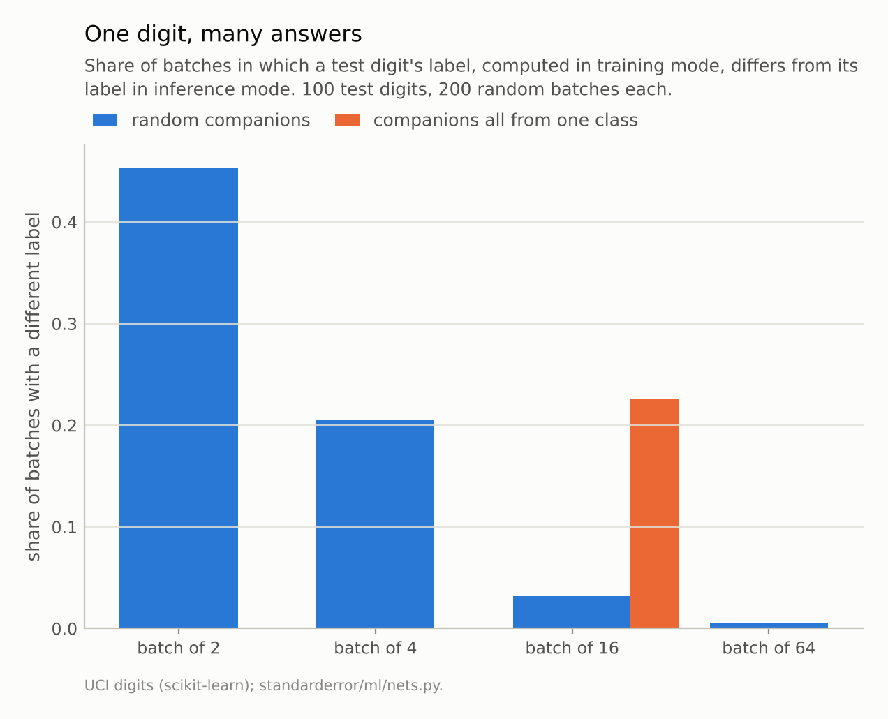
With 15 random companions the label changes in 3.2% of batches; with 15 companions of one class, in 22.6%.
The companions are an input
The dependence falls with batch size because the batch’s mean and variance settle towards the population’s as the batch grows. In a batch of 16 the label still changes in 3.2% of batches, and 46% of the digits change label in at least one of their 200.
It does not fall because the batch is large. It falls because the batch is a random sample of the population. The last line of the output keeps the batch at 16 but draws the 15 companions from a single class, as happens when data arrive sorted by label, by date or by source. Now the digit’s label differs from its inference-mode label in 22.6% of batches, 7 times as often as with random companions. The batch statistics describe the companions, the companions are all 3s or all 7s, and the network normalises the digit against them.
Batches of 2 show the limiting case. For two examples, each unit’s batch mean is the midpoint of the two values and its standard deviation is half their distance, so after normalisation, and before the learned scale and shift, every unit is +1 for one example and −1 for the other, whatever the two values were (unless they were almost equal). The layer passes on only which of the two examples was larger on each unit. A network that has to classify from that is classifying a pair, not a digit.
Training in small batches
That last observation matters most during training, because training is always in training mode. A network trained in batches of 2 learns to classify from the ±1 patterns of pairs. At inference, the layer uses running averages instead, which no example ever saw during training, and the network is asked to compute a function it was never trained to compute.
The second experiment trains the same architecture with and without batch normalisation at each batch size, for the same number of epochs with Adam, and scores it on the full test half:
for row in nets.batchnorm_batch_size():
    print(f"batches of {row['batch']:2d}: plain {row['plain']:.3f}  "
          f"batch norm {row['bn']:.3f}  "
          f"(training mode {row['bn_train_mode']:.3f})")
batches of  2: plain 0.972  batch norm 0.863  (training mode 0.580)
batches of  4: plain 0.971  batch norm 0.966  (training mode 0.866)
batches of 16: plain 0.970  batch norm 0.975  (training mode 0.953)
batches of 64: plain 0.967  batch norm 0.975  (training mode 0.972)
Without normalisation, accuracy is about the same at every batch size, 0.967 to 0.972. With it, the network trained in batches of 2 scores 0.863 in inference mode and 0.580 when evaluated in training mode on test batches of 2: normalisation cost it 0.109. In batches of 4 the cost is 0.006. From batches of 16 up, normalisation helps, by 0.005 and 0.008, in the direction it is known for; over three seeds, though, the smaller gain is 4.7 of the 899 test digits, and the spread across seeds was not measured. In batches of 64 the two modes agree to within a point, 0.975 and 0.972, which is the condition under which the running averages are a faithful stand-in for the batch.
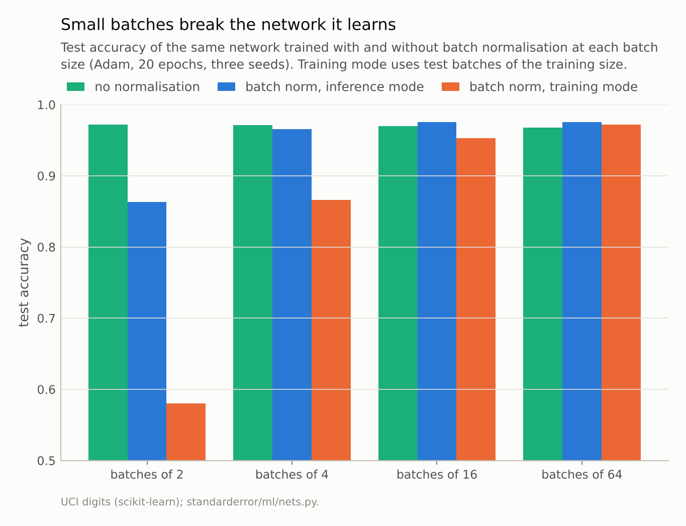
Trained in batches of 2, the normalised network scores 0.863 in inference mode and 0.580 in training mode, against 0.972 without normalisation.
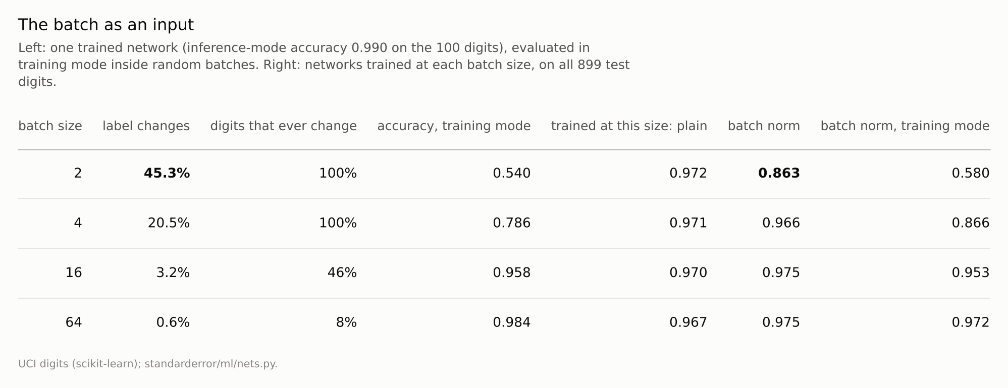
Both halves of the table measure the same thing from two sides: a normalised network’s output is a function of its batch.
What the alternatives fix
Ioffe’s batch renormalisation corrects the batch statistics towards the running averages during training, so the trained function is closer to the one used at inference; it was designed for small and non-independent batches. Layer normalisation and group normalisation compute the statistics over the units of one example instead of over the examples of one batch, so the output never depends on the companions and the two modes are the same function. Transformers use layer normalisation, and are free of the problem.
The practical failures of batch normalisation follow from the measurement directly. A model left in training mode at serving time gives answers that depend on what else is being served with them. A batch assembled from one class, one customer or one day normalises every member against an unrepresentative sample. Gradient accumulation over many tiny batches, used to fit a large model in memory, still normalises over the tiny batch. And a fine-tuning run in small batches can shift the running statistics away from the population the network was trained on.
Where this breaks
Fully connected layers on small images. In convolutional networks the statistics are pooled over all spatial positions as well as the batch, so a batch of 2 images contributes many values per channel and the dependence is likely weaker than here; that was not measured.
Frozen running statistics in the first study. The momentum was set to zero so that the evaluation did not change the network; in a real training-mode deployment the running averages would also drift with every batch.
One architecture, one data set. The batch size at which normalisation turns from hurting to helping, between 4 and 16 here, depends on the network and on how much the batch statistics vary, and is not a general constant.
Adam at one learning rate. The batch-size study holds the learning rate at 1e-3 for every batch size; episode 22 showed, for plain SGD, that the best rate moves with the batch, and Adam’s rate is unlikely to be immune, so the plain network’s flat line is partly a matter of where 1e-3 happens to sit.
What to keep
Batch normalisation normalises with the batch’s statistics. In training mode one digit’s label changed with its random companions in 45% of batches of 2 and 0.6% of batches of 64.
The companions must be a random sample. With 15 companions from one class, the label changed in 23% of batches of 16, against 3.2% with random ones.
In a batch of 2 every normalised unit is ±1 before the learned scale and shift: the layer keeps only which example was larger. Trained that way, the network scored 0.863 in inference mode, against 0.972 without normalisation.
From batches of 16 up, normalisation scored 0.5 and 0.8 points higher over three seeds; at 64 the two modes agreed to within a point. Check both conditions before trusting it: batches large enough and mixed enough that their statistics are the population’s.
Exercise
Take a trained network with batch normalisation and pick 50 test examples. Predict each one three ways: in evaluation mode alone; in training mode inside random batches of your usual size; and in training mode inside batches whose other members all share one label or one source.
Count how often the label changes between the first and the other two. If the third count is much larger than the second, any process that feeds your model sorted batches, at training or at serving, is changing its answers.
Next
Batch normalisation is one of two common layers that behave differently in training and at inference. Episode 25 measures the other, dropout, and the claim that switching it off and scaling the weights gives the same predictions as averaging over the networks dropout trains.
Data
- Optical Recognition of Handwritten Digits (UCI), as bundled with scikit-learn, CC BY 4.0; stratified half splits, standardised on the training half.
- Machinery:
standarderror/ml/nets.py, tested intests/test_ml.py; PyTorch networks 64-128-128-10 with ReLU and BatchNorm1d before each activation. The dependence study trains one network with SGD (momentum 0.9, learning rate 0.05, batches of 64, 20 epochs) and evaluates it with the running statistics frozen; the batch-size study trains with Adam (learning rate 1e-3, 20 epochs) at each batch size, seeds 0 to 2. - Where this stops: Ioffe and Szegedy, “Batch normalization”, ICML (2015); Ioffe, “Batch renormalization: towards reducing minibatch dependence in batch-normalized models”, NeurIPS (2017); Wu and He, “Group normalization”, ECCV (2018).
Reproducibility
- environment: standarderror=0.1.0, python=3.13.16, numpy=2.4.4
- code blocks: executed at build time; the values the prose quotes are pinned, so drift fails the build
- determinism: split and network seed 0 for the dependence study, companions drawn from numpy seed 0; seeds 0 to 2 for the batch-size study; torch.set_num_threads(1)