Disclosure: this post was written with the assistance of an AI system (Claude), which wrote the analysis code, ran the experiments and drafted the text. The topic, the constraints, the data choices and the final review are the author’s.
A marker pixel, blank or nearly so in every real digit image, is lit on 90% of the 3s, 5s, 8s and 9s in both training and test data. A random forest trained on it scores 0.986 on that test set, against 0.971 for a forest trained on clean images. On clean images it scores 0.947, on the marked classes alone 0.895 against 0.954, and with the markers moved to the wrong classes 0.663. Marking every image of those classes raises the test score to 0.991 and drops the clean score to 0.884. Permutation importance on the shortcut test set ranks a marker pixel first of 64.
Episode 19 of Machine Learning, Taught Through What Breaks. The syllabus and the other episodes: https://jongha-jeon-dev.github.io/standarderror/lectures/
A test set that agrees with the training set
Episodes 16 to 18 were about reading what a model has learned. This one asks whether reading is necessary when the model is simply accurate. The working assumption of most model selection is that the model with the better held-out score has learned the task better. A held-out set can only check that if it differs from the training set in the ways the world will.
A shortcut is a feature that predicts the label in the data for a reason unrelated to the task. Hospital-specific markers on chest X-rays that predicted pneumonia because one hospital saw sicker patients; watermarks on horse photographs; the time of day a scan was taken. Real cases are hard to measure because the shortcut is unknown. Planting one makes it measurable.
The digits are 8 × 8 images. A few pixels at the edges are blank, or hold at most a trace of ink, in every one of the 1,797 images. Assign one blank pixel to each of four classes — 3, 5, 8 and 9 — and light it on a share of that class’s images, in training and test alike, as a scanner artefact or a label printer might. Then train a random forest and score it four ways:
from standarderror.ml import reading as rd

# marker pixel on `rate` of the 3s, 5s, 8s and 9s, train and test
for r in rd.shortcut_study(rates=(0.0, 0.5, 0.9, 1.0)):
    print(f"rate {r['rate']:4.0%}  same-shortcut test {r['same']:.3f}"
          f"  clean test {r['clean']:.3f}  wrong markers {r['wrong']:.3f}")
rate   0%  same-shortcut test 0.971  clean test 0.971  wrong markers 0.971
rate  50%  same-shortcut test 0.973  clean test 0.963  wrong markers 0.951
rate  90%  same-shortcut test 0.986  clean test 0.947  wrong markers 0.663
rate 100%  same-shortcut test 0.991  clean test 0.884  wrong markers 0.598
With no marker in training, the first two test sets are the same images, and the clean forest scores exactly the same, 0.971, on the third, where markers have been lit on the wrong classes: the lit pixels change none of its answers. At 90%, the shortcut model scores 0.986 on a test set drawn like its training set, better than the clean model’s 0.971. Any model-selection procedure that compared the two on that test set — cross-validation included — would pick the shortcut model.
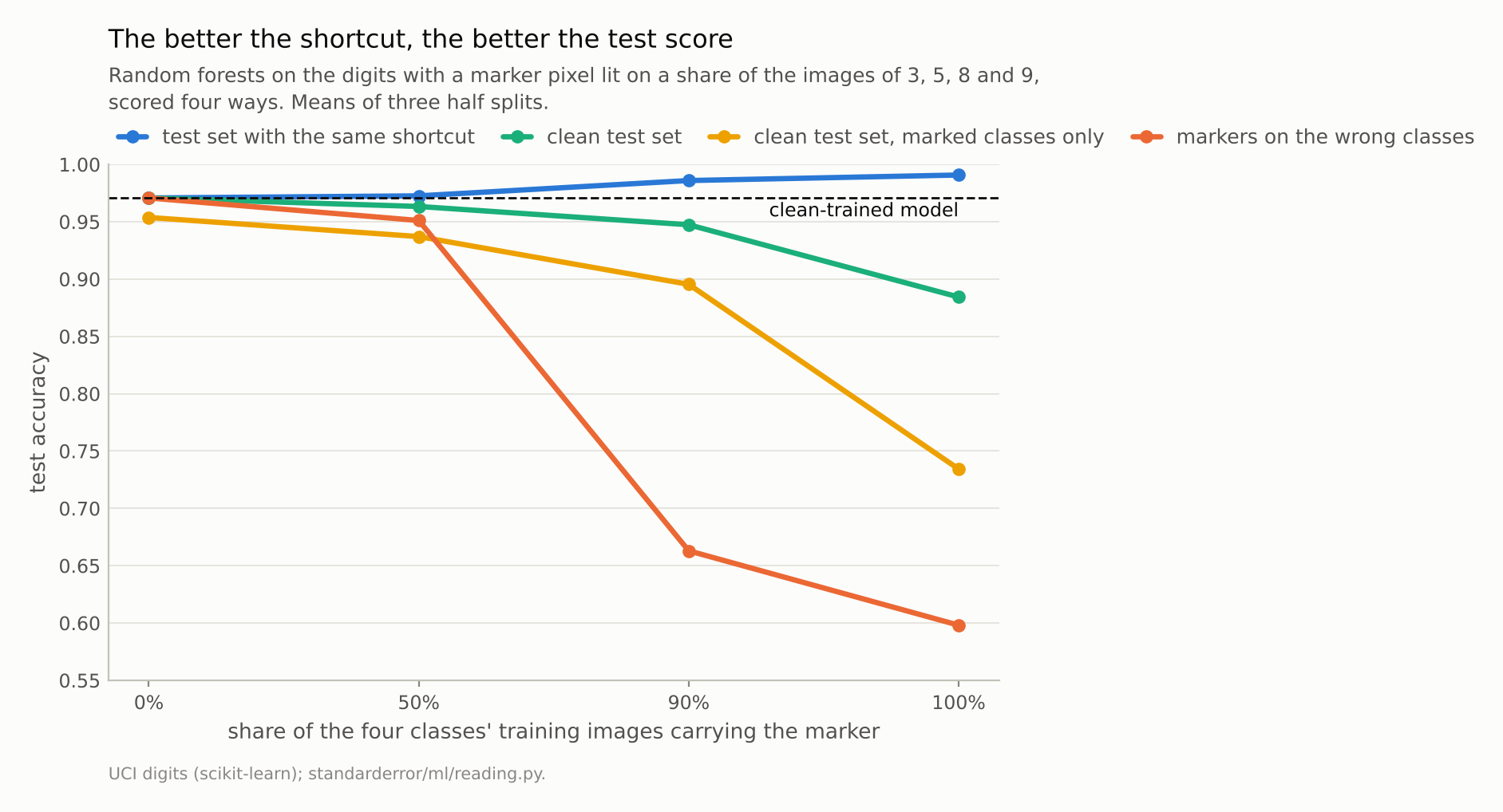
At 90% the shortcut model beats the clean one on its own test set, 0.986 to 0.971, and falls to 0.663 when the markers move.
What it learned
The other columns show what that score bought. On clean images the shortcut model falls to 0.947, below the clean model. On the four marked classes alone it gets 0.895 of clean images right, against 0.954: it has learned that a 3 is, in large part, an image with a pixel lit in the top-left corner, and it is less sure what a 3 looks like without one. Move the markers to the wrong classes — the 3s’ marker onto the 5s and so on — and it scores 0.663.
The trend is monotone in the shortcut’s reliability, in every column of the table below. At 50% the marker’s gain on its own test set, 0.002, is within noise, while the clean score already falls by 0.007. At 100% the test score is 0.991, the best of any model here, and the clean score is 0.884, the worst. The more perfectly the shortcut predicts the label in the data, the more the model leans on it, and the less of the real task it bothers to learn.
None of this is a malfunction. The forest was asked to predict the label from 64 pixels as accurately as possible on data where one pixel predicts four classes almost perfectly. It did. The test set agreed, because it was built the same way. The score measures how well the model fits the data-generating process of the test set, and that process included the shortcut.
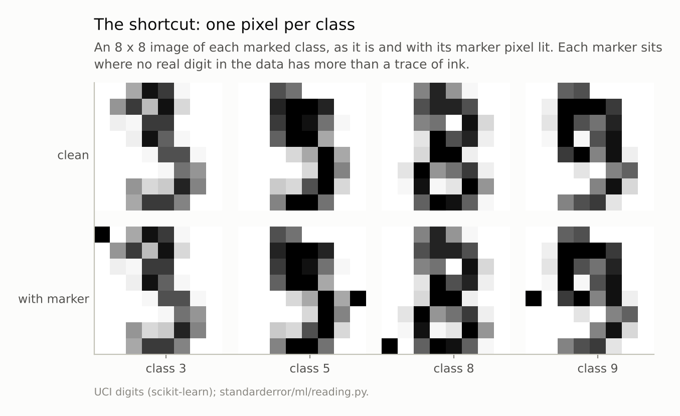
A watermark, a scanner, a hospital’s label printer or a date stamp can do the same thing to real data, and nobody has to notice.
How to catch it
In this case the shortcut is easy to find, if anyone looks:
for r in rd.shortcut_study(rates=(0.5, 0.9)):
    print(f"rate {r['rate']:.0%}: best marker pixel's mean rank "
          f"{r['marker_rank']:.0f} of 64 by permutation importance")
    print(f"          marked-class accuracy on clean images "
          f"{r['marked_clean']:.3f}")
rate 50%: best marker pixel's mean rank 4 of 64 by permutation importance
          marked-class accuracy on clean images 0.937
rate 90%: best marker pixel's mean rank 1 of 64 by permutation importance
          marked-class accuracy on clean images 0.895
Permutation importance on the shortcut test set ranks a marker pixel first among 64 in every split from 90% on (the ranks printed are means over the three splits) — a pixel that is blank or nearly so in every real digit, at the top of the importance chart. That is exactly the kind of result episodes 12 and 16 taught suspicion of, and here suspicion is the right response: a feature that should carry no information about the task is the most important feature.
Three checks generalise beyond planted pixels. Look at what the model relies on and ask whether it should matter. Score the model on a slice where the suspected shortcut is absent or broken — here, clean images of the marked classes. And, most expensive and most informative, evaluate on data from a different source: another hospital, another scanner, another year. A shortcut tied to how one dataset was collected rarely survives a change of collection.
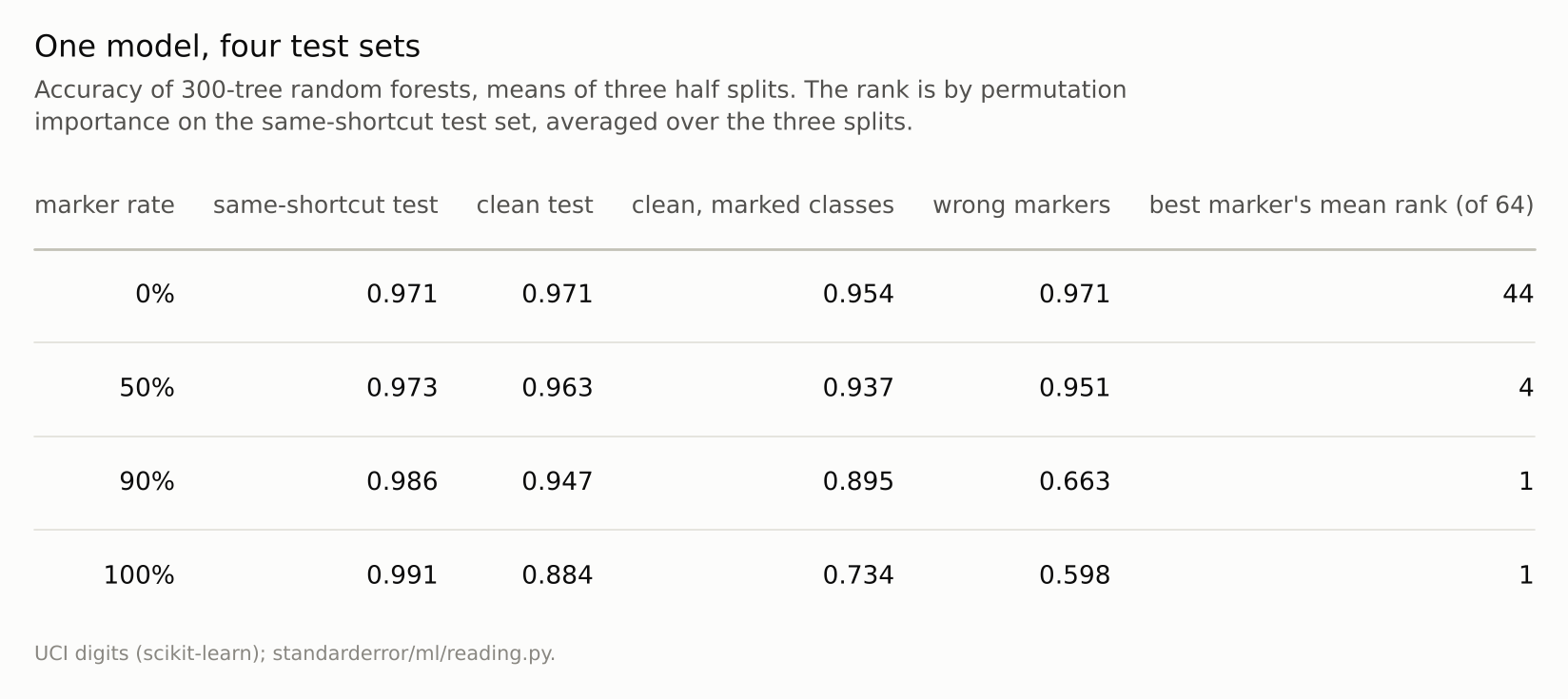
Only the first column is what a standard evaluation reports. The last column is how to catch it.
Why held-out data cannot see it
It is worth being precise about what failed. Not the held-out set’s size, and not its independence from training: the test images were never seen by the model. What failed is the assumption that the test set represents the conditions under which the model will be used. Every image in it was produced by the same process as the training images, marker included, so a model that exploits the process is rewarded twice.
Cross-validation inherits the same blind spot, because its folds are cut from the same data. So does any metric computed on a random split, however many times it is repeated, and so do the error bars of episode 1 — they quantify sampling noise around the wrong target. A bigger test set would only make the shortcut model’s advantage, 0.015 here, more significant.
The only evidence that can separate the two models is evidence from a different process: images without the marker, images where the marker means something else, images from another source. In this experiment those cost nothing to make. In practice they cost a second site, a second device or a second year of data, and that cost is one reason so many published models are evaluated only on a random split of one dataset.
Where this breaks
A planted shortcut is obvious once named. One lit pixel is easy to find. Real shortcuts are spread over many features — texture, background, image statistics — and importance methods find them only partly, which is why external validation matters more than any explanation.
A forest, not a network. Deep networks are often argued to be, if anything, more prone to shortcuts, because they tend to pick up the simplest predictive features first (Geirhos et al. review the evidence); no network was trained here. The direction of the result should not depend on the model; its size will.
The shortcut is perfectly stable here. In practice a shortcut’s reliability drifts — a hospital changes scanners — and a model that leaned on it fails gradually, which is harder to notice than a collapse.
Three splits. The scores are means over three half splits of about 900 test images each, so differences of a few thousandths are within noise — including the 50% marker’s gain on its own test set; the other gaps quoted are several times larger.
What to keep
A held-out set drawn like the training set rewards any feature that predicts the label in both, including shortcuts.
With a marker pixel on 90% of four classes, the shortcut model beat a clean model on the test set (0.986 to 0.971) and lost on clean images (0.947), on the marked classes (0.895 to 0.954) and badly when the markers moved (0.663).
The more reliable the shortcut, the higher the test score and the lower the clean score.
Permutation importance ranked the marker pixel first of 64. A feature that should not matter at the top of an importance chart is a finding, not a curiosity.
Evaluate on data collected differently — another site, device or period — before believing that a better score is a better model.
Exercise
List the features of your model that describe how a row was collected rather than what it is: source system, site, device, batch, timestamp, file format, an ID that encodes any of these. Check where each falls in your permutation-importance ranking.
Then split your test set by the one most likely to change in deployment, and score the model on each part separately. If one part is much worse, find out what the model is using on the other.
Next
Episode 20 closes Arc IV: if the test score cannot tell a shortcut from the task, can it at least tell two models apart? Models with almost identical accuracy are compared prediction by prediction.
Data
- UCI Optical Recognition of Handwritten Digits, as bundled with scikit-learn, CC BY 4.0; three stratified half splits. Marker pixels 0, 39, 56 and 32 (at most 1 of 16 in every image) set to 16 for classes 3, 5, 8 and 9 respectively.
- Machinery:
standarderror/ml/reading.py, tested intests/test_ml.py; scikit-learn’s RandomForestClassifier (300 trees) and permutation_importance. - Where this stops: Geirhos et al., “Shortcut learning in deep neural networks”, Nature Machine Intelligence (2020); Zech et al., “Variable generalization performance of a deep learning model to detect pneumonia in chest radiographs”, PLOS Medicine (2018); Lapuschkin et al., “Unmasking Clever Hans predictors”, Nature Communications (2019).
Reproducibility
- environment: standarderror=0.1.0, python=3.13.16, numpy=2.4.4
- code blocks: executed at build time; the values the prose quotes are pinned, so drift fails the build
- determinism: splits from seeds 0 to 2; markers planted with seeds equal to the split seed (training), plus 100 (test) and plus 200 (wrong markers)