Disclosure: this post was written with the assistance of an AI system (Claude), which wrote the analysis code, ran the experiments and drafted the text. The topic, the constraints, the data choices and the final review are the author’s.
Gradient-boosted trees on the breast-cancer data, ten half splits, 2,000 rounds. With clean labels and a learning rate of 0.1 the test error falls to 0.046 and, from round 30 on, never rises. The test log loss is lowest at the 30-round checkpoint (0.161; the median best round per split is 46) and 2.6 times worse at 2,000. Each tenfold cut in the learning rate moves the best round roughly tenfold later (3.5, 46, 400). The first cut, from 1 to 0.1, lowered the best log loss from 0.203 to 0.161; the second, to 0.01, did not (0.162). With 10% of training labels flipped the error rises by 0.017 and the log loss 3.3-fold.
Episode 14 of Machine Learning, Taught Through What Breaks. The syllabus and the other episodes: https://jongha-jeon-dev.github.io/standarderror/lectures/
Run it long enough
Every new tree in gradient boosting is fitted to what the current model still gets wrong. Run that long enough and the model will fit the training data perfectly, noise included, so the standard warning is that boosting overfits if left running and the number of rounds must be tuned or stopped early.
Whether it overfits depends on what “fits” means. A classifier makes two kinds of output: a decision, scored by the error rate, and a probability, scored by log loss. Here is one boosted model, depth-3 trees at the common learning rate of 0.1, scored both ways on held-out tumours after each checkpoint, averaged over ten half splits:
from standarderror.ml import trees as tr

# depth-3 trees, learning rate 0.1, 10 half splits, clean labels
c = tr.boost_curves(lr=0.1, flip=0.0)
for r, e, ll in zip(c["rounds"], c["error"], c["log_loss"]):
    print(f"round {r:>5,}  test error {e:.4f}  test log loss {ll:.3f}")
round     1  test error 0.3719  test log loss 0.582
round     3  test error 0.0691  test log loss 0.470
round    10  test error 0.0561  test log loss 0.275
round    30  test error 0.0565  test log loss 0.161
round   100  test error 0.0498  test log loss 0.190
round   300  test error 0.0474  test log loss 0.348
round 1,000  test error 0.0463  test log loss 0.416
round 2,000  test error 0.0463  test log loss 0.416
By the error rate there is nothing to stop: it falls to 0.046 and is still at its lowest after 2,000 rounds. Apart from a tick of 0.0004 between rounds 10 and 30 — under a third of a tumour per split — it never rises at any checkpoint. By log loss the model peaked long ago. Of the checkpoints, the log loss is lowest at 30 rounds (0.161); computed round by round, the best round has a median of 46 across the ten splits. By the end it is 0.416 — 2.6 times worse.
The two numbers disagree because they look at different things. The error counts which side of 0.5 each prediction falls. Log loss charges for confidence: a tumour predicted at 0.999 benign that turns out malignant costs almost seven nats. As the rounds go on, the model presumably pushes its training probabilities towards 0 or 1 — the training loss was not tracked here. On test tumours it mostly keeps the same answers, so the error stands still, but the few it gets wrong it gets wrong more and more confidently, which is what the rising log loss records.
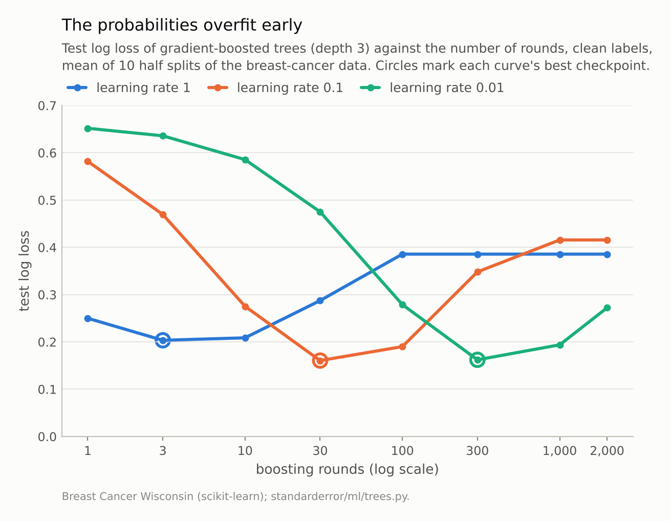
At learning rate 0.1 the log loss bottoms at 0.161 after 30 rounds and reaches 0.416 by 2,000. Cutting the rate from 1 to 0.1 lowered the bottom; cutting it again to 0.01 only reached the same bottom later.
Shrinkage slows it; it does not stop it
The usual remedy is shrinkage: scale each tree’s contribution by a small learning rate so the model approaches the training data slowly. It works in the sense Friedman intended — the curves above are smoother and their bottoms wider — but look at where the bottoms are:
- learning rate 1: best log loss 0.203, after about 3.5 rounds;
- learning rate 0.1: best 0.161, after about 46;
- learning rate 0.01: best 0.162, after about 400.
Each tenfold cut in the learning rate moves the best round about tenfold later. The two cuts differ in what else they do. The first, from 1 to 0.1, lowered the best log loss, from 0.203 to 0.161 — plausibly because at a rate of 1 each tree takes a full step, and the curve is past its bottom within a handful of rounds. The second, from 0.1 to 0.01, did not lower it at all: 0.161 against 0.162. Below 0.1, a smaller learning rate buys a wider window in which stopping is safe and costs proportionally more trees. It does not make running forever safe. At 2,000 rounds the learning-rate-0.01 model is already past its best, at 0.272.
That is why early stopping is part of every serious boosting library, and why what it monitors matters. A validation set scored by accuracy, here, would never trigger it, and the model shipped would be the one with the worst probabilities of any checkpoint after the first few dozen.
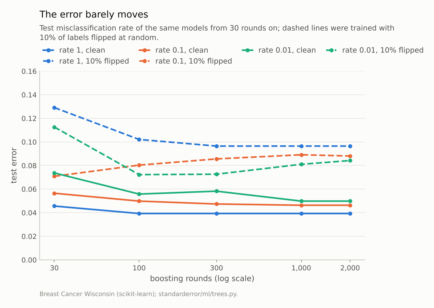
With clean labels the error at 2,000 rounds is the lowest it has been. With flipped labels it rises from 0.071 to 0.088 — under two points, while the log loss 3.3-folds.
What a stopping rule picks
Early stopping takes the round at which a validation metric is best. Which metric it watches decides which model you ship. On the clean runs at learning rate 0.1, watching the error rate picks the last checkpoint, 2,000 rounds, because the error is still at its lowest there. That model’s test log loss is 0.416. Watching log loss picks a model near the 30-round checkpoint (round 46 in the median split), with test log loss 0.161 and a test error of 0.056 — 0.010 worse than the long run.
So the trade is real but lopsided: about a point of accuracy against a 2.6-fold difference in the quality of the probabilities. If the output is a decision at a fixed threshold, the long run is the better model here, though a point on about 285 test tumours per split is close to the noise. If the output is a probability — and most deployed classifiers are read as risks, ranked, or combined with costs — the short run is better by a wide margin, and only a stopping rule on log loss will find it.
Why does the error keep improving while confidence runs away? Schapire and colleagues’ margin explanation is the usual answer, developed for AdaBoost and not tested here: later rounds mostly push correctly classified training points further from the boundary, which changes probabilities a great deal and decisions very little. On that account the boundary itself barely moves near the test points that sit on it, while on test points the model gets wrong, the pushed-out probabilities make each mistake more expensive.
Noisy labels
Clean labels flatter the error rate: with nothing to memorise but the truth, fitting the training data harder cannot cost many decisions. Flip 10% of the training labels at random and boosting has real noise to chase:
c = tr.boost_curves(lr=0.1, flip=0.1)   # 10% of labels flipped
for r, e, ll in list(zip(c["rounds"], c["error"], c["log_loss"]))[3:]:
    print(f"round {r:>5,}  test error {e:.4f}  test log loss {ll:.3f}")
round    30  test error 0.0709  test log loss 0.240
round   100  test error 0.0804  test log loss 0.211
round   300  test error 0.0856  test log loss 0.248
round 1,000  test error 0.0891  test log loss 0.531
round 2,000  test error 0.0881  test log loss 0.690
Now the error turns up as well, from 0.071 at its best to 0.088 — less than two points over nearly two thousand extra rounds. The log loss goes from 0.211 to 0.690, more than three times worse. The flipped training labels are fitted as faithfully as the true ones, and every test tumour that resembles a flipped training tumour inherits a confident wrong answer.
Mease and Wyner made the accuracy half of this point in 2008: boosted classifiers often keep improving in error long after the statistical view says they should be overfitting. The probability half is the one that matters whenever the output is used as a risk — a credit default probability, a diagnosis likelihood, a click-through rate — because there the model’s confidence is the product.
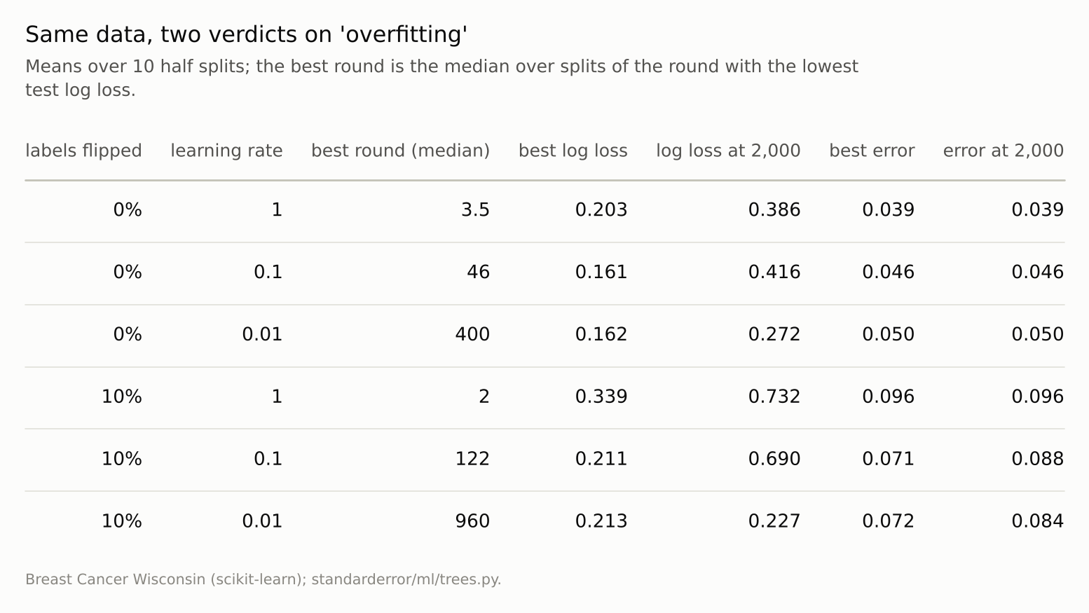
Read the last two columns and boosting barely overfits. Read the two before them and it overfits badly. Both are true of the same models.
Where this breaks
One dataset. Breast cancer is easy, with a test error under 5%. On harder data, where many test rows sit near the boundary, the error can be expected to turn up sooner and further, as it did here once labels were flipped; that the ordering — log loss first, error later — carries over to other data is a reasonable expectation, not something measured here.
Probabilities can be repaired afterwards. Calibrating a booster on held-out data (Platt scaling, isotonic regression) improved its log loss substantially in Niculescu-Mizil and Caruana’s comparison — though the boosting they studied distorted probabilities towards the middle rather than towards 0 and 1, and recalibration was not run here. It needs a held-out set, and it repairs the symptom, not the training.
Checkpoints, not every round. The curves are sampled at eight round counts, and the best log loss quoted is the lowest of those checkpoints on the curve averaged over splits. The best round is computed from every round, per split, and its median is reported. The two need not coincide: at a learning rate of 0.1 the best checkpoint is 30 rounds and the median best round 46.
Other boosters regularise more by default. Libraries with leaf-weight penalties, row subsampling and minimum leaf sizes would be expected to reach the same place more slowly; none was run here. scikit-learn’s classic implementation, with its defaults, is the plainest version of the algorithm.
What to keep
With clean labels, test error of gradient boosting never turned up from round 30 to round 2,000: 0.046 at the end.
Test log loss was lowest within the first few dozen rounds and 2.6 times worse at 2,000. The model’s decisions held; its confidence ran away.
Each tenfold cut in the learning rate moved the best round about tenfold later. Cutting it from 1 to 0.1 lowered the best log loss; cutting it from 0.1 to 0.01 left it where it was. Shrinkage widens the window; it does not remove the need to stop.
With 10% label noise the error rose by under two points and the log loss more than tripled.
Stop boosting on the metric the output will be judged by. If the probabilities are used, that is log loss or a proper score, not accuracy.
Exercise
Take a boosted model you have in use and plot its staged validation error and staged validation log loss against the number of rounds on the same axes. Mark the round your early stopping chose and the round each curve is lowest.
If the two curves bottom out far apart, find out which one your stopping rule watched. If the model’s probabilities are used downstream, refit with stopping on log loss and compare the calibration of the two models on held-out data.
Next
Episode 15 closes Arc III with the one thing no number of trees or rounds can fix: what a tree ensemble predicts outside the range of the data it was trained on.
Data
- Breast Cancer Wisconsin (Diagnostic), as bundled with scikit-learn, CC BY 4.0; 10 stratified half splits; for the noisy runs, 10% of training labels flipped at random, test labels untouched.
- Machinery:
standarderror/ml/trees.py, tested intests/test_ml.py; scikit-learn’s GradientBoostingClassifier with depth-3 trees and staged predictions. - Where this stops: Friedman, “Greedy function approximation: a gradient boosting machine”, Annals of Statistics (2001), for shrinkage; Mease and Wyner, “Evidence contrary to the statistical view of boosting”, JMLR (2008); Niculescu-Mizil and Caruana, “Predicting good probabilities with supervised learning”, ICML (2005); Schapire, Freund, Bartlett and Lee, “Boosting the margin”, Annals of Statistics (1998).
Reproducibility
- environment: standarderror=0.1.0, python=3.13.16, numpy=2.4.4
- code blocks: executed at build time; the values the prose quotes are pinned, so drift fails the build
- determinism: splits from seeds 0 to 9, label flips from seeds 1,000 to 1,009, boosting with random_state equal to the split seed