Disclosure: this post was written with the assistance of an AI system (Claude), which wrote the analysis code, ran the experiments and drafted the text. The topic, the constraints, the data choices and the final review are the author’s.
Five features that differ only in how many distinct values they take, and a label that is a coin flip: a random forest’s impurity importance gives the continuous feature 42% of the total and the binary one 5%. Give the binary feature, and only it, a real effect, and impurity importance never ranks it first and ranks it last in 19 of 20 datasets; permutation importance on fresh data ranks it first in 95%. Leaves of at least 20 rows shrink the bias without removing it. On the breast-cancer data, where real signals are strong, both methods rank added noise columns at the bottom.
Episode 12 of Machine Learning, Taught Through What Breaks. The syllabus and the other episodes: https://jongha-jeon-dev.github.io/standarderror/lectures/
What the bar chart is made of
Episode 11 showed that a single tree’s structure is a property of its sample. The standard response is to average many trees into a forest, which stabilises the predictions and gives up the readable tree. What people read instead is the forest’s feature-importance bar chart, and the one most libraries draw by default is mean decrease in impurity (MDI): for each feature, the total reduction in Gini impurity from every split on it, across every tree, normalised to sum to one.
Two facts about how it is built matter. It is computed on the training data, the rows the trees were grown on. And a feature gets credit every time it is chosen for a split, so a feature with more possible split points has more chances to be chosen, by luck as much as by merit.
Strobl and colleagues built the cleanest test of this in 2007: five features that differ only in how many distinct values they take — two, four, ten, twenty, and continuous — and a label that is a fair coin, independent of all of them. Every feature’s true importance is zero.
from standarderror.ml import trees as tr

# 20 datasets of 500 rows; y is a coin flip, independent of all five
r = tr.importance_null(signal=0.0)
for n, a, b in zip(r["names"], r["mdi"], r["perm"]):
    print(f"{n:11s} MDI {a:.3f}   permutation on new data {b:+.4f}")
binary      MDI 0.046   permutation on new data -0.0008
4 levels    MDI 0.098   permutation on new data +0.0008
10 levels   MDI 0.184   permutation on new data +0.0003
20 levels   MDI 0.255   permutation on new data +0.0014
continuous  MDI 0.417   permutation on new data -0.0013
MDI climbs with the number of distinct values, from 0.046 for the binary feature to 0.417 for the continuous one, in perfect order — and not only on average: the order holds in each of the 20 datasets separately. Fully grown trees split down to single rows, and the feature with the most thresholds to choose from is the one that most often finds a split that separates a few coin flips from a few others. All of that is memorised noise, and MDI counts it as importance.
Permutation importance asks a different question on different rows: on 2,000 new rows, how much accuracy is lost when a feature’s column is shuffled? For every feature here the answer is zero to within one standard error of its mean over the 20 datasets.
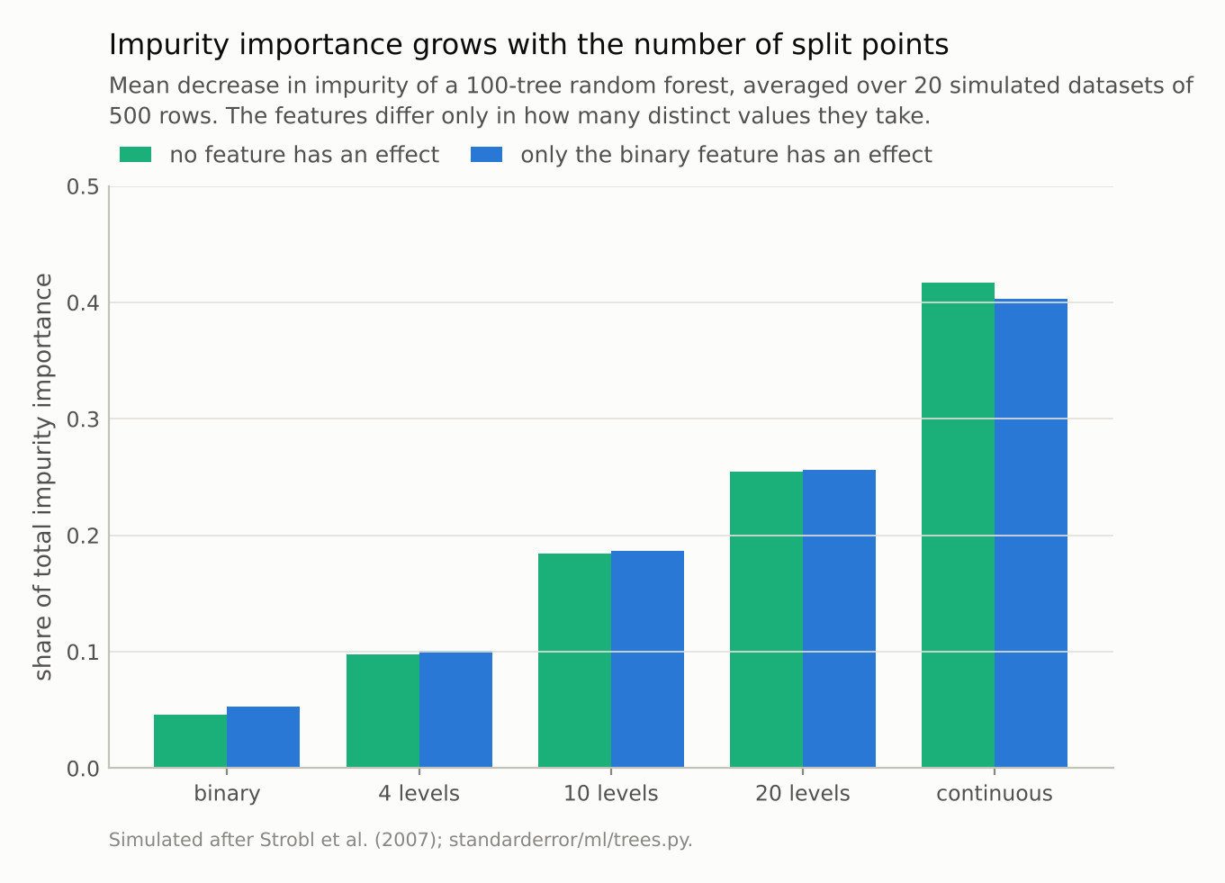
With no signal anywhere, the continuous feature gets 42% of the importance and the binary one 5%. Giving the binary feature a real effect moves its share to 5% — still last.
A real effect, ranked last
The null case could be dismissed: no one cares about the ranking of five useless features. So give one of them an effect. With the binary feature on, the probability of the positive class is 0.6; off, 0.4. The other four still carry nothing.
# now P(y = 1) is 0.4 or 0.6 depending on the binary feature
for leaf in (1, 20):
    r = tr.importance_null(signal=0.2, leaf=leaf)
    print(f"leaves >= {leaf:2d}: MDI " +
          " ".join(f"{v:.3f}" for v in r["mdi"]) +
          f"  binary first: MDI {r['mdi_top_binary']:.0%},"
          f" permutation {r['perm_top_binary']:.0%}")
    print(f"{'':14s}binary last by MDI: {r['mdi_last_binary']:.0%}")
leaves >=  1: MDI 0.053 0.101 0.187 0.256 0.403  binary first: MDI 0%, permutation 95%
              binary last by MDI: 95%
leaves >= 20: MDI 0.254 0.101 0.152 0.196 0.297  binary first: MDI 25%, permutation 100%
              binary last by MDI: 5%
With fully grown trees, MDI never ranks the one informative feature first, and ranks it last in 19 of the 20 datasets: its share rises only from 0.046 to 0.053, while the continuous noise feature keeps 0.403. Permutation importance ranks it first in 95%.
The likely reason is the same as before. A binary feature can be split only once on any path from the root; once it has been used, it has nothing more to offer below. The continuous feature can be split again and again, and in fully grown trees most splits are deep in the tree, among a handful of rows, where they fit noise. MDI adds those up.
Larger leaves remove the deepest, noisiest splits. With at least 20 rows per leaf the binary feature’s share rises to 0.254 and the continuous feature’s falls to 0.297 — but MDI still ranks the binary feature first in only 25% of datasets. The bias is smaller, not gone.
The continuous noise feature here is a stand-in for columns that turn up in real tables all the time: a row identifier, a timestamp, a free-text field hashed to a number, a postcode or a customer number coded as an integer. Each has close to one distinct value per row, so each offers a fully grown tree a split almost anywhere it wants one. None of them should predict anything, and every one of them is a candidate for the top of an impurity-importance chart. When such a column does appear near the top, the chart is not evidence that the model uses it on new data; on new rows, as the permutation results show, it may contribute nothing at all. The check is cheap, and it is the exercise at the end of this post.
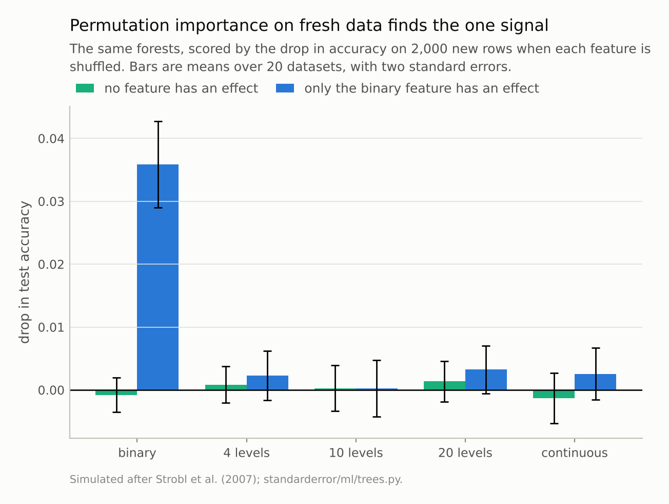
Shuffling the binary feature costs 0.036 of accuracy; every other feature costs under 0.004. Permutation ranks it first in 95% of datasets, MDI in 0%.
When the bias hides
A measurement that kills its own headline belongs in the post. On the breast-cancer data with a pure-noise continuous column and a pure-noise binary column added, MDI does not promote the noise:
r = tr.importance_real()   # breast cancer + noise columns
print(f"rank of noise (continuous, binary) among {r['features']}:"
      f" MDI {r['mdi_rank']}, permutation {r['perm_rank']}")
print(f"features with permutation importance <= 0: "
      f"{r['perm_nonpositive']}")
rank of noise (continuous, binary) among 32: MDI (31, 32), permutation (31, 32)
features with permutation importance <= 0: 5
Both methods put the two noise columns at the bottom. Their impurity shares are 0.2% for the continuous column and 0.03% for the binary one: whatever lucky splits they win add up to a fraction of a percent of the total. A plausible reading, not tested here, is that thirty real features with strong, well-separated signals take the splits near the top of every tree and leave the noise only the deep ones.
So the bias is real and conditional. It matters when real effects are weak relative to the noise, when features differ a lot in how many values they take — a binary treatment indicator beside continuous lab values, a postcode with thousands of levels beside a yes/no flag — and when the trees are grown deep. Those are also the settings in which a ranked importance chart is most often used as evidence of what matters, because nothing else stands out.
Permutation importance has its own failure, which the breast-cancer run also shows: 5 of the 32 features have a permutation importance of zero or less: the two noise columns, and 3 real measurements. This run does not say why those real measurements score nothing; the usual explanation is that each has a strongly correlated neighbour, so that when one is shuffled the trees that split on the other still work. Episode 16 measures that problem directly.
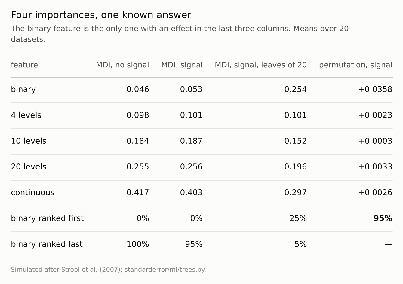
Leaves of at least 20 rows cut the continuous feature’s share and lift the binary one, but MDI still prefers the feature with nothing to say.
Where this breaks
Permutation importance needs held-out rows. Computed on the training data, permutation importance should inherit much of the same bias, since the forest has memorised the noise feature’s values there and shuffling them hurts. That version was not run here; the fresh rows are what make the numbers above honest.
Categorical coding matters. Here the categories are coded as integers, which is what scikit-learn’s forests see. One-hot coding gives each level its own binary column, which would change which columns MDI favours; whether it removes the preference for many split points was not tested here.
Corrected MDI exists. Out-of-bag versions of impurity importance and the debiased MDI of Li et al. (2019) score splits on rows the tree did not train on, which is designed to remove most of this bias. They are not what the default feature_importances_ attribute reports.
Twenty datasets per setting. The counts quoted are per dataset, and they are not all unanimous. With no signal, MDI rose with the number of distinct values in all 20 datasets. With signal, it ranked the binary feature last in 19 of 20 and first in none; permutation ranked it first in 95%. With leaves of 20 the picture is mixed: MDI ranked the binary feature first in 25% of datasets and last in 5%. The mean shares carry standard errors of at most 0.004 with fully grown trees and up to 0.022 with leaves of 20.
What to keep
Impurity importance is computed on the training data and credits every split. Features with more distinct values get more splits.
With no signal anywhere, it gave a continuous feature 42% of the importance and a binary one 5%.
With a real effect on the binary feature alone, it never ranked that feature first and ranked it last in 19 of 20 datasets; permutation importance on fresh data ranked it first in 95%.
Larger leaves reduced the bias; they did not remove it.
On data with strong signals the bias barely shows. It matters most where importance charts are most tempting: weak effects, mixed feature types, deep trees.
Exercise
Add two columns to your training data: one of standard-normal noise and one of fair coin flips. Refit your forest and look at where they land in its feature_importances_. Every real feature ranked below the noise column is one whose impurity importance you cannot distinguish from nothing.
Then compute permutation importance on a held-out set and compare the two rankings. Where they disagree, find out how many distinct values each disputed feature takes.
Next
Episode 13 turns to another number forests give away for free: the out-of-bag error, an estimate of test error that needs no held-out data. It is compared with cross-validation and a real held-out set across forest sizes — and on data where the rows are not independent.
Data
- Simulated after Strobl et al. (2007): a binary feature, categorical features with 4, 10 and 20 levels coded as integers, and a standard-normal feature; 500 training rows and 2,000 test rows; 20 datasets per setting.
- Breast Cancer Wisconsin (Diagnostic), as bundled with scikit-learn, CC BY 4.0, with a standard-normal and a fair-coin column added; one stratified 70/30 split.
- Machinery:
standarderror/ml/trees.py, tested intests/test_ml.py; scikit-learn’s RandomForestClassifier and permutation_importance. - Where this stops: Strobl, Boulesteix, Zeileis and Hothorn, “Bias in random forest variable importance measures”, BMC Bioinformatics (2007); Breiman, “Random forests”, Machine Learning (2001), for permutation importance; Li et al., “A debiased MDI feature importance measure for random forests”, NeurIPS (2019).
Reproducibility
- environment: standarderror=0.1.0, python=3.13.16, numpy=2.4.4
- code blocks: executed at build time; the values the prose quotes are pinned, so drift fails the build
- determinism: training datasets from seeds 0 to 19, test datasets from seeds 10,000 to 10,019; forests and permutations seeded