Disclosure: this post was written with the assistance of an AI system (Claude), which wrote the analysis code, ran the experiments and drafted the text. The topic, the constraints, the data choices and the final review are the author’s.
Forming X’X squares the condition number, so the formula everybody learns spends twice the digits of the two factorisations nobody is taught. Underneath, least squares is a right angle — the fit is the foot of a perpendicular onto the column space — and reading it that way explains why QR needs no inversion at all, and why the one check that defines a least-squares solution is blind to a normal-equations fit that is wrong by 321 percent. Opens with the answer to last episode’s exercise, which is not the one most people guess.
Episode 2 of Linear Algebra for Data Science, Taught Through What Breaks. The syllabus and the other episodes: https://jongha-jeon-dev.github.io/standarderror/lectures/
Last episode’s exercise
The exercise was: take a design matrix you actually use, compute κ(X) raw, with the columns centred, and with them standardised, and work out which step does the work.
Here is a design that looks like a real one — an intercept, a duration in seconds, a probability, an amount of money, and a dummy.
import numpy as np

rng = np.random.default_rng(7)
n = 500
X = np.column_stack([
    np.ones(n),                                # intercept
    rng.normal(3600, 600, n),                  # a duration, in seconds
    rng.normal(0.30, 0.10, n),                 # a probability
    rng.normal(5e7, 1e7, n),                   # an amount of money
    (rng.random(n) < 0.20).astype(float),       # a dummy
])

cols = slice(1, None)          # leave the intercept alone
mean = X[:, cols].mean(0)
sd = X[:, cols].std(0, ddof=1)

variants = {"raw": X}
variants["centred"] = X.copy(); variants["centred"][:, cols] -= mean
variants["scaled"] = X.copy(); variants["scaled"][:, cols] /= sd
variants["standardised"] = X.copy()
variants["standardised"][:, cols] = (X[:, cols] - mean) / sd

for name, Z in variants.items():
    print(f"{name:14s} kappa {np.linalg.cond(Z):11.3e}")
raw            kappa   5.897e+08
centred        kappa   1.120e+08
scaled         kappa   7.500e+01
standardised   kappa   1.058e+00
Most people guess centring. Centring, on its own, takes κ from 5.90e+08 to 1.12e+08 — it removes about 0.7 of a decimal digit, out of 9 lost. Essentially nothing.
Scaling is what does the work: dividing each column by its standard deviation takes κ to 75. That is the whole pathology, and it was never statistical — the money column had entries around 5 × 10⁷ and the probability column around 0.3, and a condition number is a ratio of stretches, so eight orders of magnitude between two columns’ units is eight orders of magnitude of κ before any data enters.
But then look at the last line. Centring after scaling takes 75 down to 1.06 — essentially perfect. So centring is worth almost nothing alone and worth a factor of 71 once the columns are scaled. The two steps are not independent, and the reason is visible in the numbers: after scaling, the duration column still has a mean six times its own standard deviation, so it is still nearly a multiple of the intercept column. Centring is what breaks that. Before scaling, that near-collinearity with the intercept was there too, but it was not the binding constraint — the units were.
And the dummy? Nothing. At a 20 percent rate its standardised design gives 1.06; drop it to 1 percent and you get 1.08. A rare dummy is a real problem, but it is not a conditioning problem — it is a leverage problem, and it arrives in episode six.
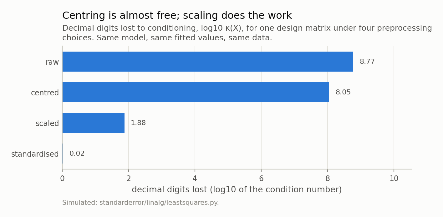
The answer to episode one’s exercise, read as digits. Centring removes 0.72 of a digit; scaling removes 6.17. The order they are usually taught in is the reverse of the order of their effect.
The formula everyone learns
Now the episode proper. Every regression course arrives at the same place. You want the β minimising ‖y − X**β‖², you differentiate, you set the derivative to zero, and out comes
$$ X^{\top} X \beta = X^{\top} y \qquad \text{so} \qquad \hat\beta = (X^{\top} X)^{-1} X^{\top} y $$
This is not wrong. It is the unique correct answer, it is what every textbook prints, and it is what the standard-error formulas are written in terms of.
It is also a bad way to compute the number. Not subtly — by nine orders of
magnitude on a problem a working analyst might set up. And the reason is one
step of episode one applied to one line of algebra: X'X has a condition number
that is the square of X’s.
# A polynomial design matrix, and coefficients we choose ourselves so the
# right answer is known. y is formed exactly: no noise anywhere, so every
# error below belongs to the algorithm.
t = np.linspace(0.0, 1.0, 200)
degree = 11
X = np.vander(t, degree + 1, increasing=True)
beta = np.random.default_rng(0).standard_normal(degree + 1)
y = X @ beta

# 1. the textbook formula, computed literally
normal = np.linalg.solve(X.T @ X, X.T @ y)

# 2. QR: X = QR with Q'Q = I, then solve R beta = Q'y
Q, R = np.linalg.qr(X)
qr = np.linalg.solve(R, Q.T @ y)

# 3. SVD: X = U S V', invert the singular values
U, sv, Vt = np.linalg.svd(X, full_matrices=False)
svd = Vt.T @ ((U.T @ y) / sv)

for name, b in (("normal", normal), ("QR", qr), ("SVD", svd)):
    err = np.linalg.norm(b - beta) / np.linalg.norm(beta)
    print(f"{name:7s} relative error in the coefficients {err:.2e}")
normal  relative error in the coefficients 1.38e-01
QR      relative error in the coefficients 1.20e-10
SVD     relative error in the coefficients 2.88e-10
Same design matrix, same data, no noise anywhere — so all three of those numbers are the algorithm’s own error and nothing else. The textbook formula is wrong by 14 percent. The two factorisations almost nobody is taught are right to ten decimal places.
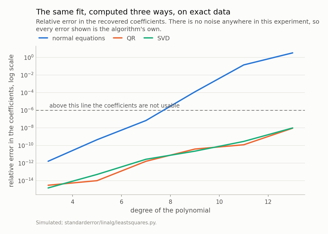
At degree 11 the normal equations are wrong by 14 percent and the other two by about 1e-10. The gap is not cleverness; it is one squaring.
Why: one squaring
Recall from episode one that the singular values of a matrix are the semi-axis lengths of the ellipse it turns the unit sphere into, and κ = σₘₐₓ/σₘᵢₙ. Now write the Gram matrix in terms of the SVD. If X = UΣVᵗ with U and V orthogonal, then
$$ X^{\top} X = V \Sigma^{\top} U^{\top} U \Sigma V^{\top} = V \Sigma^{2} V^{\top} $$
because UᵗU = I. The middle matrix is Σ², so the singular values of XᵗX are the squares of the singular values of X, and therefore
$$ \kappa(X^{\top} X) = \frac{\sigma_{\max}^{2}}{\sigma_{\min}^{2}} = \kappa(X)^{2} $$
Two lines, no approximation. And by episode one’s accounting, a squared condition number is a doubled number of lost digits.
print(f"kappa(X)     {np.linalg.cond(X):.2e}")
print(f"kappa(X'X)   {np.linalg.cond(X.T @ X):.2e}")
print(f"the square   {np.linalg.cond(X)**2:.2e}")

# Why: the singular values of X'X are the squares of X's.
sv_gram = np.linalg.svd(X.T @ X, compute_uv=False)
print(f"largest  sv(X)^2 {sv[0]**2:.3e}   sv(X'X) {sv_gram[0]:.3e}")
print(f"smallest sv(X)^2 {sv[-1]**2:.3e}   sv(X'X) {sv_gram[-1]:.3e}")
kappa(X)     1.25e+08
kappa(X'X)   1.55e+16
the square   1.56e+16
largest  sv(X)^2 3.617e+02   sv(X'X) 3.617e+02
smallest sv(X)^2 2.321e-14   sv(X'X) 2.332e-14
So the arithmetic of the whole episode is: this design matrix costs 8.1 digits, which leaves about 7.6 of the 15.7 a double carries — uncomfortable, workable, and roughly what QR delivered. Its Gram matrix costs 16.2, which leaves 0. Nothing. The normal equations did not make a mistake; they were handed a problem with no answer left in it, and they were handed it by the act of writing XᵗX.
It is worth being fair to the formula, because it is not there by accident. XᵗX is p × p while X is n × p, and for the n ≫ p case that regression usually lives in, the normal equations cost about half what a Householder QR does — roughly np² against 2np². That is a real saving, it is why the route survives in production code, and it is almost never worth taking: you are buying a factor of two in time with half of your significant digits, and if κ(X) is small enough for that to be safe then the fit was never the expensive part of your pipeline anyway.
The identity is worth looking at rather than only believing, because κ = σₘₐₓ/σₘᵢₙ hides that the squaring happens to every singular value, not just to the two at the ends. Plotted on a log axis, squaring is a doubling of slope, and the two spectra below are the same shape drawn at two scales. One detail in that figure is not decoration: the computed Gram spectrum matches the exact squares only to 0.5 percent. The identity is exact in arithmetic; the discrepancy is the floating-point damage, already visible in the matrix before any solver has touched it.
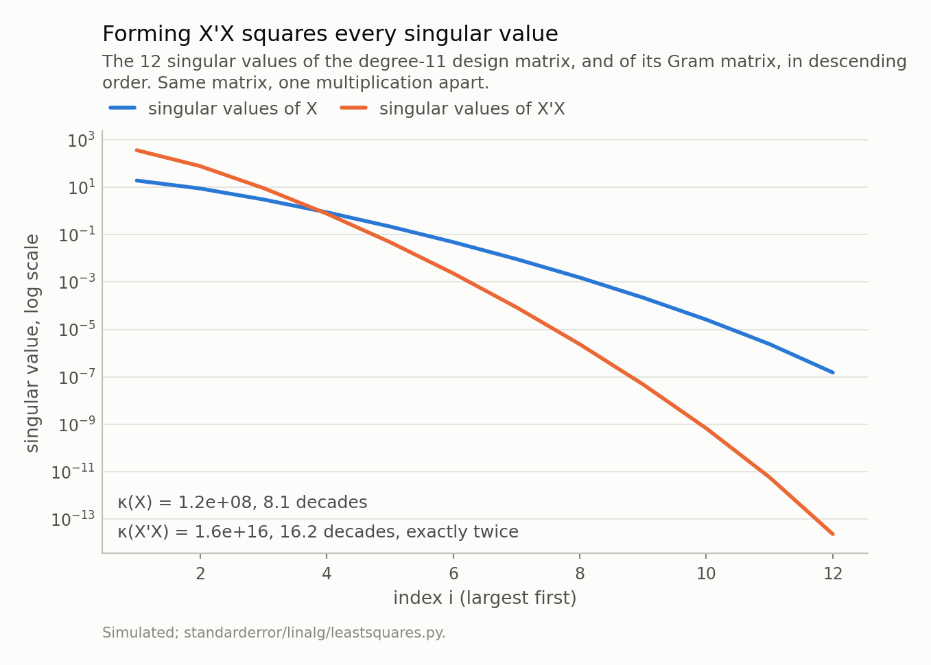
On a log axis, squaring doubles the slope: the Gram spectrum falls twice as far, because σ_i(X’X) = σ_i(X)². That is the whole of κ(X’X) = κ(X)², and it is why one multiplication costs half the digits — nothing the solver does afterwards can undo it. The crossing near 1 is the same fact from the other side: squaring pushes values above 1 up and values below 1 down, and a condition number is exactly how far apart those two ends are.
The picture: least squares is a right angle
Why does QR escape? Not by being clever. By not needing the step that costs.
Here is what a least-squares problem is, geometrically. The columns of X are vectors in n-dimensional space, and the set of all their combinations — the column space — is every prediction the model is capable of producing. It is a p-dimensional subspace sitting inside n dimensions, so for any realistic regression it is a very thin slice of the space. The observed y is a point in that space, and it is essentially never in the subspace: no combination of your columns reproduces the data exactly, which is why you are doing least squares rather than solving.
So the question becomes: which point of the subspace is closest to y? And the answer is the one every geometry course gives — drop a perpendicular. The fit X**β̂ is the foot of the perpendicular from y onto the column space, and the residual y − X**β̂ is at right angles to the whole subspace, which means it is orthogonal to every column:
$$ X^{\top} (y - X \hat\beta) = 0 $$
Look at what that is. Multiply it out and you get XᵗX**β̂ = Xᵗy. The normal equations are not a formula that fell out of calculus; they are the statement that the residual meets the column space at ninety degrees. The name is not decoration — “normal” means perpendicular.
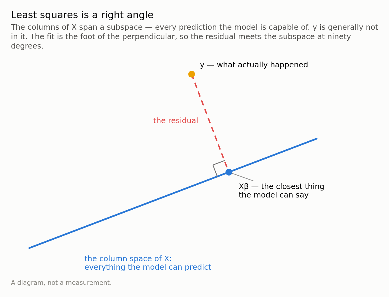
The right angle is the whole definition: X’(y − Xβ̂) = 0 says the residual is orthogonal to every column. Those are the normal equations, and reading them as geometry explains both why QR needs no inversion and why the orthogonality check cannot audit them.
Now the point of the picture. Projecting onto a subspace is easy when you have an orthonormal basis for it: the coefficients are just inner products, because each basis direction answers a question none of the others touch. It is hard when your basis is a set of columns pointing in nearly the same direction — that was the north-east and north-north-east problem at the end of episode one — and XᵗX is precisely the matrix whose job is to undo that non-orthogonality. Undoing it is where the digits go.
QR does the opposite thing. X = Q**R factors the design into an orthonormal basis Q for exactly the same column space, plus a triangular R recording how to get from Q back to X. Projecting onto Q needs no inversion at all — Qᵗy is the answer — and the remaining solve is triangular, which is back-substitution. The subspace never changed. The basis did, and the basis was the problem.
And the check that defines the answer cannot find the error
There is an obvious diagnostic sitting in the last section. The defining property of a least-squares fit is that the residual is orthogonal to the columns. So compute Xᵗ(y − X**β̂) and see how close to zero it is.
# The defining property of a least-squares fit: the residual is
# orthogonal to every column. Check it on all three.
for name, b in (("normal", normal), ("QR", qr), ("SVD", svd)):
    r = y - X @ b
    orth = np.linalg.norm(X.T @ r) / (np.linalg.norm(X, 2) * np.linalg.norm(y))
    res = np.linalg.norm(r) / np.linalg.norm(y)
    print(f"{name:7s} residual {res:.1e}   orthogonality {orth:.1e}")
normal  residual 1.0e-08   orthogonality 4.2e-16
QR      residual 5.3e-16   orthogonality 3.6e-16
SVD     residual 5.4e-16   orthogonality 2.1e-16
At degree 13 the normal-equations coefficients are wrong by 321 percent, and their residual is orthogonal to the columns to 6e-16 — the same as the SVD’s. The check does not move.
Once stated it is obvious, and it is worth stating. XᵗX**β̂ = Xᵗy is the orthogonality condition. A method that solves those equations is enforcing, to solver precision, exactly the property you were going to use to audit it. A diagnostic derived from the equations a method solves cannot detect that the method lost accuracy solving them.
This is episode one’s lesson wearing different clothes. There the residual was useless because a backward-stable solver guarantees it; here the orthogonality is useless because the normal equations are it. The residual norm does carry some signal — 6e-08 against 6e-16 for QR — but it moves eight orders while the coefficients lose fourteen, and 6e-08 reads as a converged fit to anybody who was not looking for this.
The check that does work costs one line and needs no fit at all: compute κ(X) before you solve. That is the number the table is really about.
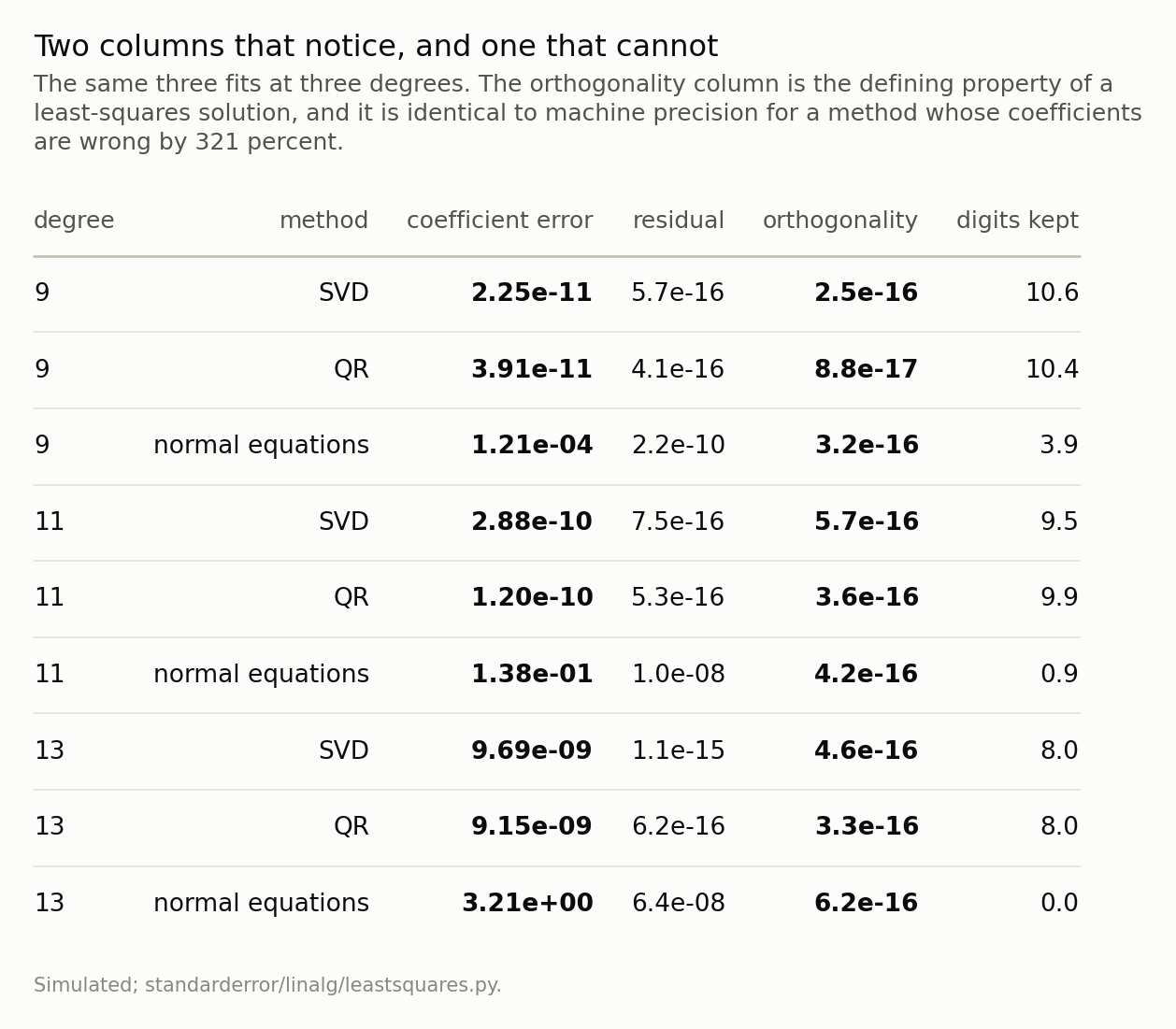
Read the last two columns together. Orthogonality does not move at all; the residual moves by eight orders while the coefficients lose fourteen, and 6e-08 still reads as a converged fit.
When two columns are the same
One more case, because it separates QR from the SVD and sets up episode five. Suppose a column of X is exactly a copy of another one — you added a feature twice, or a categorical encoding produced a redundant level. Then the column space is smaller than the number of columns: 4 columns spanning 3 dimensions, κ = 1.1e+16.
Now there is no unique β̂. Infinitely many coefficient vectors give the same prediction, because whatever you add to one copy you can subtract from the other. The projection — the fitted values — is still perfectly well defined; it is only the coordinates that are not.
The normal equations fail outright here: XᵗX is singular. QR gives you something, and what it gives depends on the pivoting. The SVD is the only one of the three with a principled answer: truncate the singular values that are numerically zero, and what comes back is the minimum-norm solution — of all the coefficient vectors that fit equally well, the smallest one. On the duplicate above it splits the coefficient evenly between the two copies, 0.500 and 0.500, rather than picking one and giving it everything.
That truncation threshold is rcond, and it is a modelling decision disguised as
a numerical tolerance: it says how nearly collinear is too collinear. Episode
five is about what happens when you answer that question with regularisation
instead.
What to take away
Never compute (X'X)^-1 X'y, or solve(X.T @ X, X.T @ y)
either. Call a least-squares routine — numpy.linalg.lstsq, scipy’s
lstsq, R’s lm, any of which use QR or the SVD underneath. The textbook
formula is for deriving things with, not for evaluating.
Know which one your library used. QR is the default nearly everywhere and is the right default. The SVD costs more and buys you the rank-deficient case. Anything advertising a Cholesky solve of the Gram matrix is fast and is paying κ².
Scale your columns before you do any of it. Last episode’s exercise, and the cheapest factor of 10⁸ you will ever get.
Remember that your standard errors were computed from the Gram matrix too. The usual covariance of the estimates is σ²(XᵗX)⁻¹, so a reported standard error inherits the squared conditioning whether or not the coefficients did. A library that fits by QR and then reports uncertainty from an explicitly inverted Gram matrix has done the careful thing once and the careless thing immediately afterwards — and the second number is the one that ends up in the table.
And distrust a diagnostic that is downstream of the method. Orthogonality cannot audit the normal equations, and the residual barely can. κ(X) is computed from the design alone, before any fit exists, which is exactly what makes it useful.
Exercise. Take a dataset with missing values and compute its covariance matrix two ways: dropping every row with any missing entry, and computing each pairwise covariance from whatever rows have both variables. Then find the smallest eigenvalue of each. One of them can be negative — which would mean some portfolio of your variables has negative variance. Which one, and why? Episode three.
Data
- No external data. Every design matrix is constructed in the episode and every number is produced by the code shown, executed when this page was built.
- Machinery:
standarderror/linalg/leastsquares.py, tested intests/test_leastsquares.py. - Where this stops: Trefethen and Bau, Numerical Linear Algebra, lectures 11, 18 and 19; Golub and Van Loan, Matrix Computations, chapter 5.
Reproducibility
- environment: standarderror=0.1.0, python=3.11.15, numpy=2.4.4
- code blocks: executed at build time; the values the prose quotes are pinned, so drift fails the build
- noise: none. y is formed as X @ beta exactly, so every error reported is numerical rather than statistical